Working with vectors

Many of R’s most useful functions process vectors of numbers in some way. For example (as we’ve already seen) if we want to calculate the average of our vector of heights we just type:

mean(heights)
[1] 167.6923

R contains lots of built in functions which we can use to summarise a vector of numbers. For example:

median(heights)
[1] 167
sd(heights)
[1] 17.59443
min(heights)
[1] 134
max(heights)
[1] 203
range(heights)
[1] 134 203
IQR(heights)
[1] 17
length(heights)
[1] 13

All of these functions accept a vector as input, do some proccesing, and then return a single number which gets displayed by RStudio.

But not all functions return a single number in the way that mean did above. Some return a new vector, or some other type of object instead. For example, the quantile function returns the values at the 0, 25th, 50th, 75th and 100th percentiles (by default).

height.quantiles <- quantile(heights)
height.quantiles
  0%  25%  50%  75% 100% 
 134  158  167  175  203

If a function returns a vector, we can use it just like any other vector:

height.quantiles <- quantile(heights)

# grab the third element, which is the median
height.quantiles[3]
50% 
167 

# assign the first element to a variable
min.height <- height.quantiles[1]
min.height
 0% 
134

But other functions process a vector without returning any numbers. For example, the hist function returns a histogram:

hist(heights)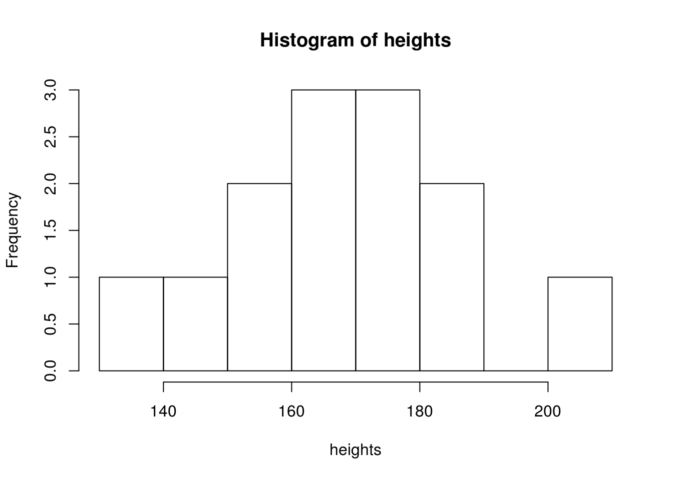

We’ll cover lots more plotting and visualisation later on.

Making new vectors

So far we’ve seen R functions which process a vector of numbers and produce a single number, a new vector of a different length (like quantile or fivenum), or some other object (like hist which makes a plot). However many other functions accept a single input, do something to it, and return a single processed value.

For example, the square root function, sqrt, accepts a single value and returns a single value: running sqrt(10) will return 3.1623.

In R, if a function accepts a single value as input and returns a single value as output (like sqrt(10)), then you can usually give a vector as input too. Some people find this surprising⁴, but R assumes that if you’re processing a vector of numbers, you want the function applied to each of them in the same way.

This turns out to be very useful. For example, let’s say we want the square root of each of the elements of our height data:

# these are the raw values
heights
 [1] 203 148 156 158 167 162 172 164 172 187 134 182 175

# takes the sqrt of each value and returns a vector of all the square roots
sqrt(heights)
 [1] 14.24781 12.16553 12.49000 12.56981 12.92285 12.72792 13.11488
 [8] 12.80625 13.11488 13.67479 11.57584 13.49074 13.22876

This also works with simple arithmetic So, if we wanted to convert all the heights from cm to meters we could just type:

heights / 100
 [1] 2.03 1.48 1.56 1.58 1.67 1.62 1.72 1.64 1.72 1.87 1.34 1.82 1.75

This trick also works with other functions like paste, which combines the inputs you send it to produce an alphanumeric string:

paste("Once", "upon", "a", "time")
[1] "Once upon a time"

If we send a vector to paste it assumes we want a vector of results, with each element in the vector pasted next to each other:

bottles <- c(100, 99, 98, "...")
paste(bottles, "green bottles hanging on the wall")
[1] "100 green bottles hanging on the wall"
[2] "99 green bottles hanging on the wall" 
[3] "98 green bottles hanging on the wall" 
[4] "... green bottles hanging on the wall"

In other programming languages we might have had to write a ‘loop’ to create each line of the song, but R lets us write short statements to summarise what needs to be done; we don’t need to worry worrying about how it gets done.

The paste0 function does much the same, but leaves no spaces in the combined strings, which can be useful:

paste0("N=", 1:10)
 [1] "N=1"  "N=2"  "N=3"  "N=4"  "N=5"  "N=6"  "N=7"  "N=8"  "N=9"  "N=10"

Making up data (new vectors)

Sometimes you’ll need to create vectors containing regular sequences or randomly selected numbers.

To create regular sequences a convenient shortcut is the ‘colon’ operator. For example, if we type 1:10 then we get a vector of numbers from 1 to 10:

1:10
 [1]  1  2  3  4  5  6  7  8  9 10

The seq function allows you to create more specific sequences:

# make a sequence, specifying the interval between them
seq(from=0.1, to=2, by=.1)
 [1] 0.1 0.2 0.3 0.4 0.5 0.6 0.7 0.8 0.9 1.0 1.1 1.2 1.3 1.4 1.5 1.6 1.7
[18] 1.8 1.9 2.0

We can also use random number-generating functions built into R to create vectors:

# 10 uniformly distributed random numbers between 0 and 1
runif(10)
 [1] 0.87168030 0.45828409 0.15508810 0.38966190 0.19589958 0.25464771
 [7] 0.31191689 0.55988519 0.57941593 0.03542701

# 1,000 uniformly distributed random numbers between 1 and 100
my.numbers <- runif(1000, 1, 10)

# 10 random-normal numbers with mean 10 and SD=1
rnorm(10, mean=10)
 [1] 10.662969 12.160476  8.229125 10.022313  8.812693 10.264308 10.030635
 [8]  9.424233 10.928984  9.602996

# 10 random-normal numbers with mean 10 and SD=5
rnorm(10, 10, 5)
 [1] 10.3415063  5.5384192  0.5174545 14.7483051  5.9846947  6.2770860
 [7] 16.5046287  7.9870762 18.4745866 12.1417264

We can then use these numbers in our code, for example plotting them:

random.numbers <- rnorm(10000)
hist(random.numbers)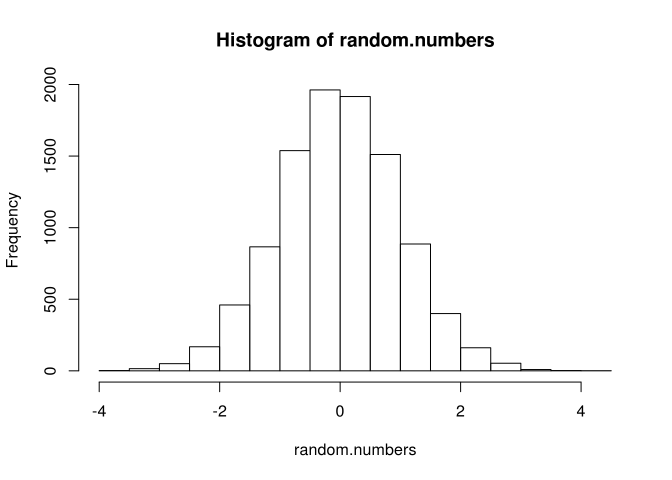

Mostly people who already know other programming languages like C. It’s not that surprising if you read the R code as you would English.↩