9 Generalized linear models
Linear regression is suitable for outcomes which are continuous numerical scores. In practice this requirement is often relaxed slightly, for example for data which are slightly skewed, or where scores are somewhat censored ( e.g. questionnaire scores which have a minium or maximum).
However, for some types of outcomes standard linear models are unsuitable. Examples here include binary (zero or one) or count data (i.e. positive integers representing frequencies), or proportions (e.g. proportion of product failures per batch). This section is primarily concerned with binary outcomes, but many of the same principles apply to these other types of outcome.
Logistic regression
In R we fit logistic regression with the glm() function which is built into R,
or if we have a multilevel model with a binary outcome we
use glmer() from the lme4:: package.
Fitting the model is very similar to linear regression, except we need to
specify the family="binomial" parameter to let R know what type of data we are
using.
Here we use the titanic dataset (you can download this from
Kaggle, although you need to sign up
for an account).
Before we start fitting models, it’s best to plot the data to give us a feel for what is happening.
Figure 1 reveals that, across all fare categories, women were more likely to survive the disaster than men. Ticket class also appears to be related to outcome: those with third class tickets were less likely to survive than those with first or second class tickets. However, differences in survival rates for men and women differed across ticket classes: women with third class tickets appear to have been less advantaged (compared to men) than women with first or second class tickets.
titanic <- read.csv('data/titanic.csv')
titanic %>%
  ggplot(aes(factor(Pclass), Survived,
             group=Sex, color=Sex)) +
  stat_summary() +
  stat_summary(geom="line") +
  xlab("Ticket class")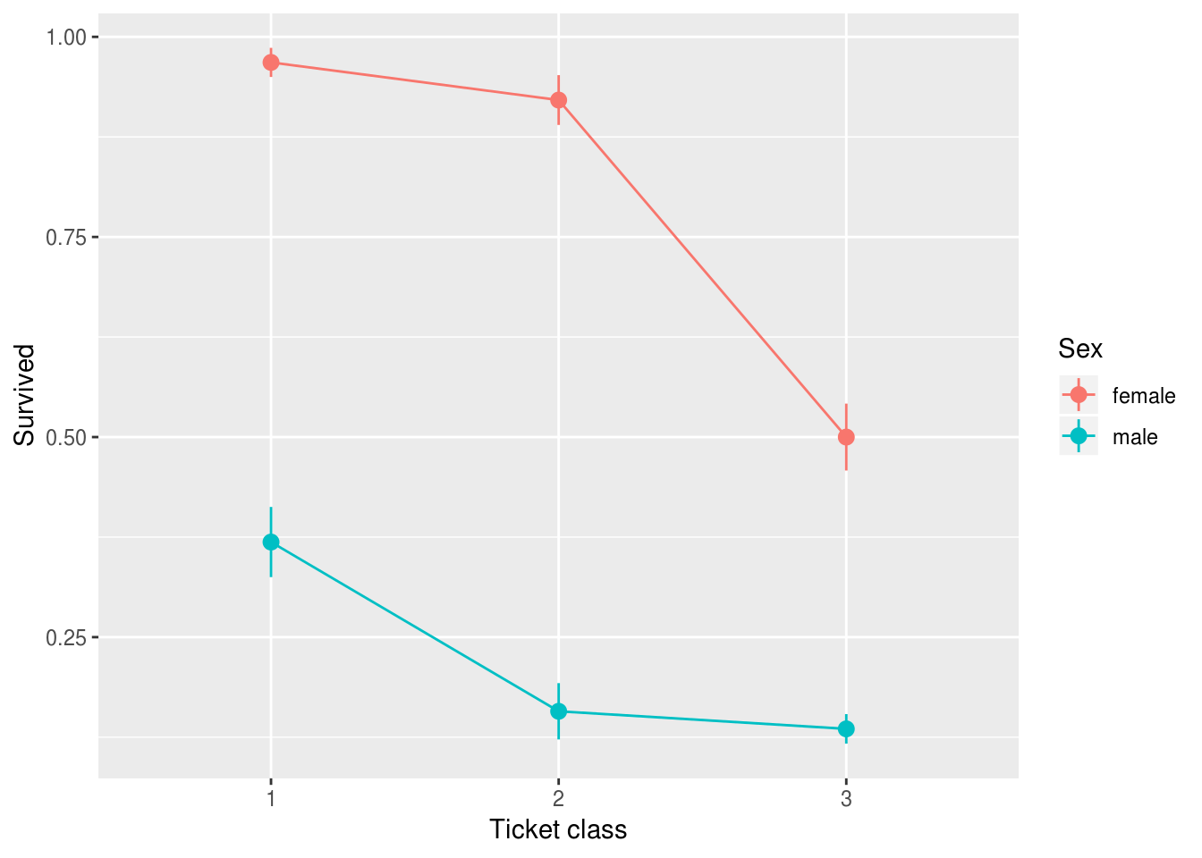
Figure 9.1: Survival probabilities by Sex and ticket class.
Given the plot above, it seems reasonable to predict survival from Sex and
Pclass, and also to include the interaction between these variables.
To run a logistic regression we specify the model as we would with lm(), but
instead use glm() and specify the family parameter:
m <- glm(Survived ~ Sex * factor(Pclass),
         data=titanic, family = binomial(link="logit"))
Because it can become repetitive to write out the family parameter in full
each time, I usually write a ‘helper function’ called
logistic() which simply calls glm with the right settings. For example:
# define a helper function for logistic regression the '...'
# means 'all arguments', so this function passes all it's
# arguments on to the glm function, but sets the family correctly
logistic <- function(...) {
  glm(..., family = binomial(link="logit"))
}
Which you can use like so:
logistic(Survived ~ Sex * factor(Pclass), data=titanic)

Call:  glm(formula = ..1, family = binomial(link = "logit"), data = ..2)

Coefficients:
            (Intercept)                  Sexmale          factor(Pclass)2
                 3.4122                  -3.9494                  -0.9555
        factor(Pclass)3  Sexmale:factor(Pclass)2  Sexmale:factor(Pclass)3
                -3.4122                  -0.1850                   2.0958

Degrees of Freedom: 890 Total (i.e. Null);  885 Residual
Null Deviance:      1187
Residual Deviance: 798.1    AIC: 810.1
Tests of parameters
As with lm() models, we can use the summary() function to get p values for
parameters in glm objects:
titanic.model <- logistic(Survived ~ Sex * factor(Pclass), data=titanic)
summary(titanic.model)

Call:
glm(formula = ..1, family = binomial(link = "logit"), data = ..2)

Deviance Residuals:
    Min       1Q   Median       3Q      Max
-2.6248  -0.5853  -0.5395   0.4056   1.9996

Coefficients:
                        Estimate Std. Error z value Pr(>|z|)
(Intercept)               3.4122     0.5868   5.815 6.06e-09 ***
Sexmale                  -3.9494     0.6161  -6.411 1.45e-10 ***
factor(Pclass)2          -0.9555     0.7248  -1.318  0.18737
factor(Pclass)3          -3.4122     0.6100  -5.594 2.22e-08 ***
Sexmale:factor(Pclass)2  -0.1850     0.7939  -0.233  0.81575
Sexmale:factor(Pclass)3   2.0958     0.6572   3.189  0.00143 **
---
Signif. codes:  0 '***' 0.001 '**' 0.01 '*' 0.05 '.' 0.1 ' ' 1

(Dispersion parameter for binomial family taken to be 1)

    Null deviance: 1186.7  on 890  degrees of freedom
Residual deviance:  798.1  on 885  degrees of freedom
AIC: 810.1

Number of Fisher Scoring iterations: 6
You might have spotted in this table that summary reports z tests rather
than t tests for parameters in the glm model. These can be interepreted as
you would the t-test in a linear model, however.
Tests of categorical predictorss
Where there are categorical predictors we can also reuse the car::Anova
function to get the equivalent of the F test from a linear model
(with type 3 sums of squares; remember not to use the built in
anova function unless you want type 1 sums of squares):
car::Anova(titanic.model, type=3)
Analysis of Deviance Table (Type III tests)

Response: Survived
                   LR Chisq Df Pr(>Chisq)
Sex                  97.547  1  < 2.2e-16 ***
factor(Pclass)       90.355  2  < 2.2e-16 ***
Sex:factor(Pclass)   28.791  2  5.598e-07 ***
---
Signif. codes:  0 '***' 0.001 '**' 0.01 '*' 0.05 '.' 0.1 ' ' 1
Note that the Anova table for a glm model provides \(\chi^2\) tests in place of
F tests. Although they are calculated differently, you can interpret these
\(\chi^2\) tests and p values as you would for F tests in a regular
Anova.
Predictions after glm
As with linear models, we can make predictions from glm models for our current
or new data.
One twist here though is that we have to choose whether to make predictions in
units of the response (i.e. probability of survival), or of the transformed
response (logit) that is actually the ‘outcome’ in a glm (see the
explainer on transformations and links functions).
You will almost always want predictions in the units of your response, which
means you need to add type="response" to the predict() function call. Here
we predict the chance of survival for a new female passenger with a first class
ticket:
new.passenger = expand.grid(Pclass=1, Sex=c("female"))
predict.glm(titanic.model, newdata=new.passenger, type="response")
        1
0.9680851
And we could plot probabilities for each gender and class with a standard error for this prediction if desired:
new.passengers = expand.grid(Pclass=1:3, Sex=c("female", "male"))

# this creates two vectors: $fit, which contains
# predicted probabilities and $se.fit
preds <- predict.glm(titanic.model,
                     newdata=new.passengers,
                     type="response",
                     se.fit=T)

new.passengers %>%
  mutate(fit = preds$fit,
         lower=fit - preds$se.fit,
         upper=fit + preds$se.fit) %>%
  ggplot(aes(factor(Pclass), fit,
             ymin=lower, ymax=upper,
             group=Sex, color=Sex)) +
  geom_pointrange() +
  geom_line() +
  xlab("Ticket class") +
  ylab("Probability of survival")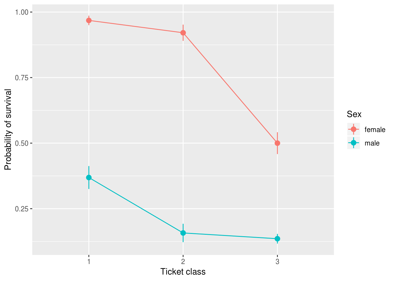
Evaluating logistic regression models
glm models don’t provide an R2 statistic, but it is possible to evaluate
how well the model fits the data in other ways.
Although there are various pseudo-R2 statistics available for glm; see
https://www.r-bloggers.com/evaluating-logistic-regression-models/
One common technique, however, is to build a model using a ‘training’ dataset (sometimes a subset of your data) and evaluate how well this model predicts new observations in a ‘test’ dataset. See http://r4ds.had.co.nz/model-assess.html for an introduction.