7 Regression
This section assumes most readers will have done an introductory statistics course and had some practice running multiple regression and or Anova in SPSS or a similar package.
Describing statistical models using formulae
R requires that you are explicit about the statistical model you want to run but
provides a neat, concise way of describing models, called a formula. For
multiple regression and simple Anova, the formulas we write map closely onto the
underlying linear model. The formula syntax provides shortcuts to quickly
describe all the models you are likely to need.
Formulas have two parts: the left hand side and the right hand side, which are
separated by the tilde symbol: ~. Here, the tilde just means ‘is predicted
by’.
For example, this formula specifies a regression model where height is the
outcome, and age and gender are the predictor variables.8
height ~ age + genderThere are lots more useful tricks to learn when writing formulas, which are covered below. But in the interests of instant gratification let’s work through a simple example first:
Running a linear model
Linear models (including Anova and multiple regression) are run using the
lm(...) function, short for ‘linear model’. We will use the mtcars dataset,
which is built into R, for our first example.
First, we have a quick look at the data. The pairs plot suggests that mpg
might be related to a number of the other variables including disp (engine
size) and wt (car weight):
mtcars %>%
  select(mpg, disp, wt) %>%
  pairs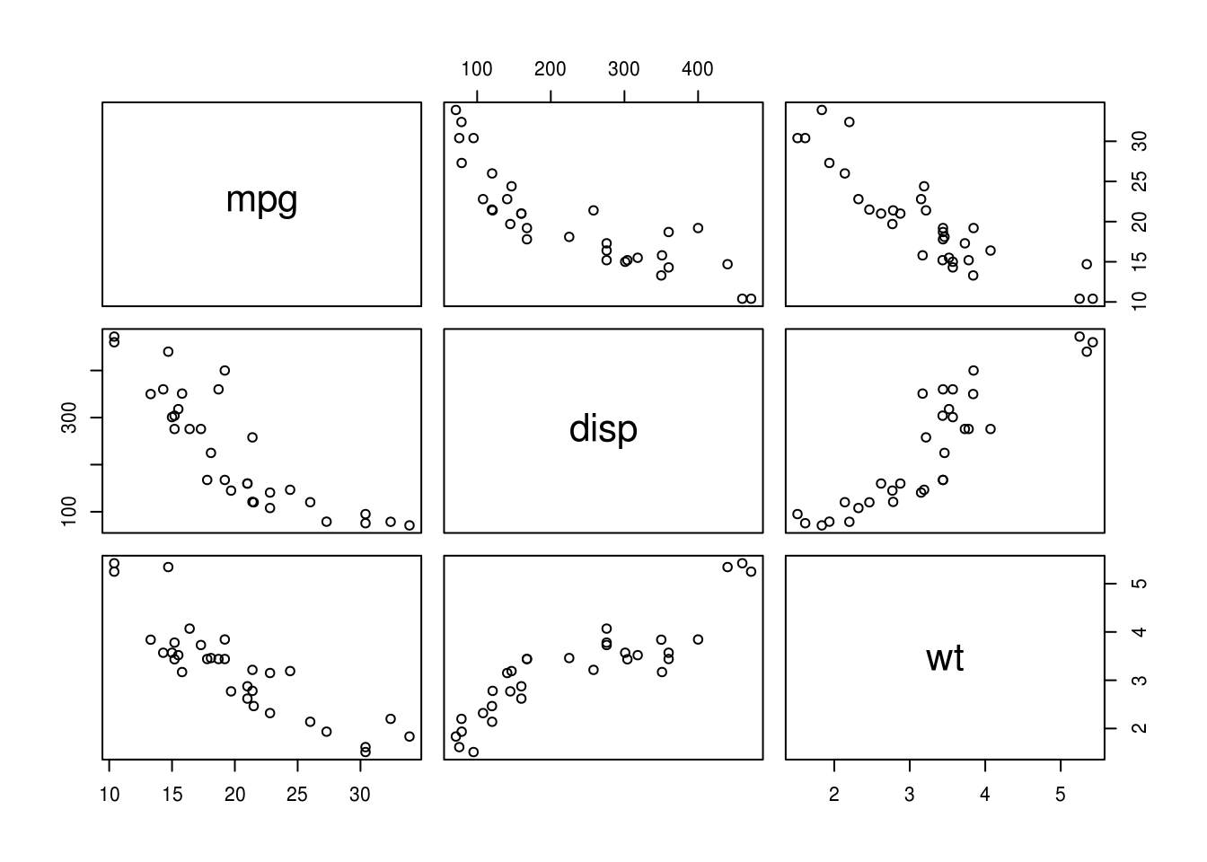
Before running any model, we should ask outselves: “what question we are trying to answer?”
In this instance, we can see that both weight (wt) and engine size (disp)
are related to mpg, but they are also correlated with one another. We might
want to know, then, “are weight and engine size independent predictors of
mpg?” That is, if we know a car’s weight, do we gain additional information
about it’s mpg by measuring engine size?
To answer this, we could use multiple regression, including both wt and disp
as predictors of mpg. The formula for this model would be mpg ~ wt + disp.
The command below runs the model:
lm(mpg ~ wt + disp, data=mtcars)

Call:
lm(formula = mpg ~ wt + disp, data = mtcars)

Coefficients:
(Intercept)           wt         disp
   34.96055     -3.35083     -0.01772
For readers used to wading through reams of SPSS output R might seem concise to
the point of rudeness. By default, the lm commands displays very little, only
repeating the formula and listing the coefficients for each predictor in the
model.
So what next? Unlike SPSS, we must be explicit and tell R exactly what we want.
The most convenient way to do this is to first store the results of the lm()
function:
m.1 <- lm(mpg ~ wt + disp, data=mtcars)This stores the results of the lm() function in a variable named m.1. As an
aside, this is a pretty terrible variable name — try to give descriptive names
to your variables because this will prevent errors and make your code easier to
read.
We can then use other functions to get more information about the model. For example:
summary(m.1)

Call:
lm(formula = mpg ~ wt + disp, data = mtcars)

Residuals:
    Min      1Q  Median      3Q     Max
-3.4087 -2.3243 -0.7683  1.7721  6.3484

Coefficients:
            Estimate Std. Error t value Pr(>|t|)
(Intercept) 34.96055    2.16454  16.151 4.91e-16 ***
wt          -3.35082    1.16413  -2.878  0.00743 **
disp        -0.01773    0.00919  -1.929  0.06362 .
---
Signif. codes:  0 '***' 0.001 '**' 0.01 '*' 0.05 '.' 0.1 ' ' 1

Residual standard error: 2.917 on 29 degrees of freedom
Multiple R-squared:  0.7809,    Adjusted R-squared:  0.7658
F-statistic: 51.69 on 2 and 29 DF,  p-value: 2.744e-10
Although still compact, the summary function provides some familiar output,
including the estimate, SE, and p value for each parameter.
Take a moment to find the following statistics in the output above:
- The coefficients and p values for each predictor
- The R2 for the overall model. What % of variance in
mpgis explained?
Answer the original question: ‘accounting for weight (wt), does engine size
(disp) tell us anything extra about a car’s mpg?’
More on formulas
Above we briefly introduced R’s formula syntax. Formulas for linear models have the following structure:
left_hand_side ~ right_hand_sideFor linear models the left side is our outcome, which is must be a continous
variable. For categorical or binary outcomes you need to use glm() function,
rather than lm(). See the section on generalised linear models)
for more details.
The right hand side of the formula lists our predictors. In the example above
we used the + symbol to separate the predictors wt and disp. This told R
to simply add each predictor to the model. However, many times we want to
specify relationships between our predictors, as well as between predictors
and outcomes.
For example, we might have an experiment with 2 categorical predictors, each with 2 levels — that is, a 2x2 between-subjects design.
Below, we define and run a linear model with both vs and am as predictors,
along with the interaction of vs:am. We save this model as m.2, and use the
summary command to print the coefficients.
m.2 <- lm(mpg ~ vs + am + vs:am, data=mtcars)
summary(m.2)

Call:
lm(formula = mpg ~ vs + am + vs:am, data = mtcars)

Residuals:
   Min     1Q Median     3Q    Max
-6.971 -1.973  0.300  2.036  6.250

Coefficients:
            Estimate Std. Error t value Pr(>|t|)
(Intercept)   15.050      1.002  15.017 6.34e-15 ***
vs             5.693      1.651   3.448   0.0018 **
am             4.700      1.736   2.708   0.0114 *
vs:am          2.929      2.541   1.153   0.2589
---
Signif. codes:  0 '***' 0.001 '**' 0.01 '*' 0.05 '.' 0.1 ' ' 1

Residual standard error: 3.472 on 28 degrees of freedom
Multiple R-squared:  0.7003,    Adjusted R-squared:  0.6682
F-statistic: 21.81 on 3 and 28 DF,  p-value: 1.735e-07
We’d normally want to see the Anova table for this model, including the F-tests:
car::Anova(m.2)
Anova Table (Type II tests)

Response: mpg
          Sum Sq Df F value    Pr(>F)
vs        367.41  1 30.4836 6.687e-06 ***
am        276.03  1 22.9021 4.984e-05 ***
vs:am      16.01  1  1.3283    0.2589
Residuals 337.48 28
---
Signif. codes:  0 '***' 0.001 '**' 0.01 '*' 0.05 '.' 0.1 ' ' 1
But before you do too much with Anova in R read this section.
Other formula shortcuts
In addition to the + symbol, we can use other shortcuts to create linear
models.
As seen above, the colon (:) operator indicates the interaction between two
terms. So a:b is equivalent to creating a new variable in the data frame where
a is multiplied by b.
The * symbol indicates the expansion of other terms in the model. So, a*b is
the equivalent of a + b + a:b.
Finally, it’s good to know that other functions can be used within R formulas to
save work. For example, if you wanted to transform your dependent variable then
log(y) ~ x will do what you might expect, and saves creating temporary
variables in your dataset.
The formula syntax is very powerful, and the above only shows the basics, but
you can read the formulae help pages in RStudio for more details.
Run the following models using the mtcars dataset:
With
mpgas the outcome, and withcylandhpas predictorsAs above, but adding the interaction of
cylandhp.Repeat the model above, but write the formula a different way (make the formula either more or less explicit, but retaining the same predictors in the model).
I avoid the terms dependent/independent variables because they are confusing to many students, and because they are misleading when discussing non-experimental data.↩