13 Power analysis
For most inferential statistics
If you want to do power analysis for a standard statistical test, e.g. t-tests,
chi2 or Anova, the pwr:: package is what you need.
This guide has a good walkthrough.
For multilevel or generalised linear models
If you’d like to run power analyses for linear mixed models
(multilevel models) then you need
the simr:: package.
It has some neat features for calculating power by simulating data and results
from a model you specify.
To take a simple example, let’s fabricate some data where outcomes y are
nested within groups g, and where there is a covariate of interest x. That
is, we are interested in estimating our power to detect an effect of x.
Note though that in this simulated data, we create outcomes (y) with no
relationship to x, and no clustering by g at this stage (i.e. y, x and
g are uncorrelated).
set.seed(1234)
simulated.df <- data_frame(
  x = rep(0:1, 50),
  g = rep(1:10, 10),
  y = rnorm(100)
)
Warning: `data_frame()` is deprecated, use `tibble()`.
This warning is displayed once per session.
GGally::ggpairs(simulated.df)
Registered S3 method overwritten by 'GGally':
  method from
  +.gg   ggplot2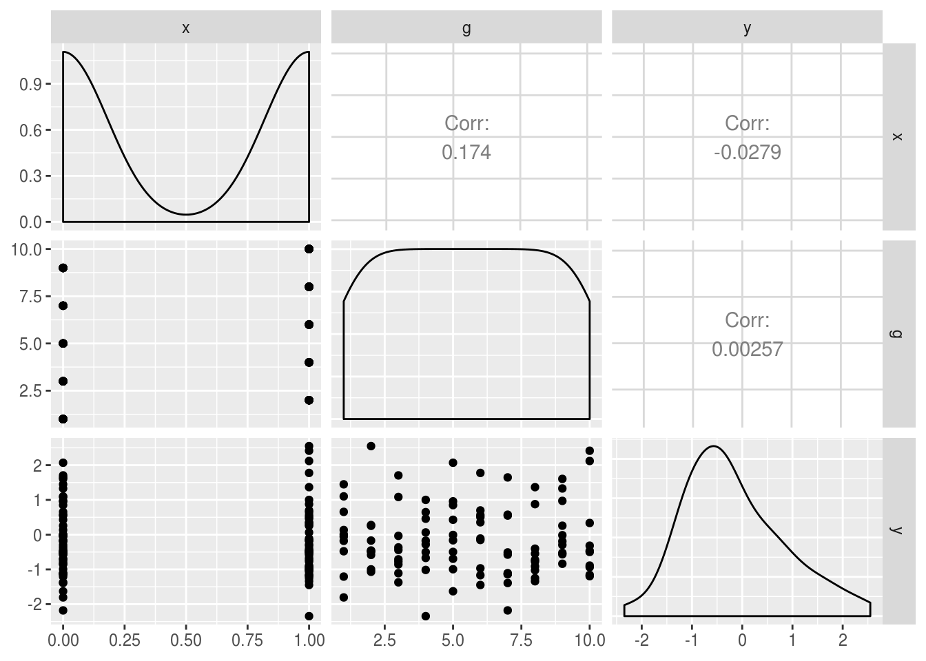
To use simr:: we first run our ‘model of interest’. In this case it’s a
random-intercepts multilevel model. We can verify x is
unrelated to outcome with lmerTest::anova:
library(lmerTest)

Attaching package: 'lmerTest'
The following object is masked from 'package:lme4':

    lmer
The following object is masked from 'package:stats':

    step
model.of.interest <- lmer(y ~ x + (1|g), data=simulated.df)
boundary (singular) fit: see ?isSingular
anova(model.of.interest)
Type III Analysis of Variance Table with Satterthwaite's method
    Sum Sq  Mean Sq NumDF DenDF F value Pr(>F)
x 0.077811 0.077811     1    98  0.0764 0.7828
The next step is to modify our saved model of interest. We tweak the fitted parameters to represent our predicted values for effect sizes, variances, and covariances.
First, let’s change the ‘true’ effect of x to be 0.2:
fixef(model.of.interest)['x'] <- .2We now use the powerSim function to use our tweaked model to:
- create a dataset using the parameters of our model (i.e. make random draws
of
ywhich relate togandxas specified in the model summary). - re-run
lmeron this simulated data. - repeat this hundreds or thousands of times
- count how many times (i.e., for what proportion) we get a significant p value
power.sim
Power for predictor 'x', (95% confidence interval):
      11.00% ( 5.62, 18.83)

Test: unknown test
      Effect size for x is 0.20

Based on 100 simulations, (1 warning, 0 errors)
alpha = 0.05, nrow = 100

Time elapsed: 0 h 0 m 11 s
Our observed power (proportion of times we get a significant p value) is very
low here, so we might want increase our hypothesised effect of x, for example
to see what power we have to detect an effect of x = .8:
fixef(model.of.interest)['x'] <- .8power.sim
Power for predictor 'x', (95% confidence interval):
95.00% (88.72, 98.36)
Test: unknown test
Effect size for x is 0.80
Based on 100 simulations, (0 warnings, 0 errors)
alpha = 0.05, nrow = 100
Time elapsed: 0 h 0 m 11 sWe might also want to set one of the variance parameters of our model to
represent clustering within-g. First we can use VarCorr() to check the
variance parameters of the model we just ran:
VarCorr(model.of.interest)
 Groups   Name        Std.Dev.
 g        (Intercept) 0.0000
 Residual             1.0091
And we could simulate increasing the variance parameter for g to 0.5:
VarCorr(model.of.interest)['g'] <- .5power.sim
Power for predictor 'x', (95% confidence interval):
33.00% (23.92, 43.12)
Test: unknown test
Effect size for x is 0.80
Based on 100 simulations, (0 warnings, 0 errors)
alpha = 0.05, nrow = 100
Time elapsed: 0 h 0 m 11 sBecause the amount of clustering in our data has increased our statistical power
has gone down. This is because, when clustering is present, each new observation
(row) in the dataset provides less new information to estimate our treatment
effect. Note that in this example we increased the variance associated with g
by quite a lot: setting the variance of g to 0.5 equates to an ICC for g of
.33 (because .5 / (.5 + 1) = .33; see the section on calculating ICCs and
VPCs)
For more details of simr see:
http://onlinelibrary.wiley.com/doi/10.1111/2041-210X.12504/full
Note that for real applications you would want to set nsim to something
reasonably large. Certainly at least 1000 simulations, and perhaps up to
~5000.