Contrasts and followup tests using lmer

Contrasts and followup tests using `lmer`

Many of the contrasts possible after lm and Anova models are also possible using lmer for multilevel models.

Let’s say we repeat one of the models used in a previous section, looking at the effect of Days of sleep deprivation on reaction times:

m <- lmer(Reaction~factor(Days)+(1|Subject), data=lme4::sleepstudy)
anova(m)
Type III Analysis of Variance Table with Satterthwaite's method
             Sum Sq Mean Sq NumDF DenDF F value    Pr(>F)    
factor(Days) 166235   18471     9   153  18.703 < 2.2e-16 ***
---
Signif. codes:  0 '***' 0.001 '**' 0.01 '*' 0.05 '.' 0.1 ' ' 1

We can see a significant effect of Days in the Anova table, and want to compute followup tests.

To first estimate cell means and create an emmeans object, you can use the emmeans() function in the emmeans:: package:

m.emm <- emmeans(m, "Days")
m.emm
 Days emmean   SE df lower.CL upper.CL
    0    257 11.5 42      234      280
    1    264 11.5 42      241      288
    2    265 11.5 42      242      288
    3    283 11.5 42      260      306
    4    289 11.5 42      266      312
    5    309 11.5 42      285      332
    6    312 11.5 42      289      335
    7    319 11.5 42      296      342
    8    337 11.5 42      314      360
    9    351 11.5 42      328      374

Degrees-of-freedom method: kenward-roger 
Confidence level used: 0.95

It might be nice to extract these estimates and plot them:

m.emm.df <-
  m.emm %>%
  broom::tidy()

m.emm.df %>%
  ggplot(aes(Days, estimate, ymin=conf.low, ymax=conf.high)) +
  geom_pointrange() +
  ylab("RT")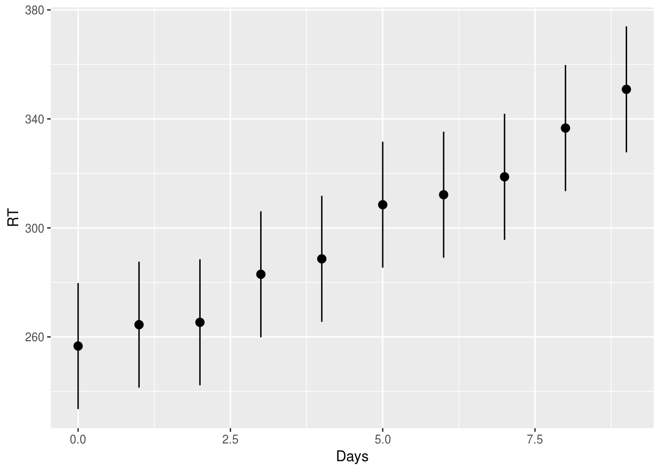

If we wanted to compare each day against every other day (i.e. all the pairwise comparisons) we can use contrast():

# results not shown to save space
contrast(m.emm, 'tukey') %>%
  broom::tidy() %>%
  head(6)

Or we might want to see if there was a significant change between any specific day and baseline:

# results not shown to save space
contrast(m.emm, 'trt.vs.ctrl') %>%
  broom::tidy() %>%
  head %>%
  pander

Perhaps more interesting in this example is to check the polynomial contrasts, to see if there was a linear or quadratic change in RT over days:

# results not shown to save space
contrast(m.emm, 'poly') %>%
  broom::tidy() %>%
  head(3) %>%
  pander(caption="The first three polynomial contrasts. Note you'd have to have quite a fancy theory to warrant looking at any of the higher level polynomial terms.")