Types of variable
When working with data in Excel or other packages like SPSS you’ve probably become aware that different types of data get treated differently.
For example, in Excel you can’t set up a formula like =SUM(...) on cells which include letters (rather than just numbers). It does’t make sensible.
However, Excel and many other programmes will sometimes make guesses about what to do if you combine different types of data.
For example, in Excel, if you add 28 to 1 Feb 2017 the result is 1 March 2017. This is sometimes what you want, but can often lead to unexpected results and errors in data analyses.
R is much more strict about not mixing types of data. Vectors (or columns in dataframes) can only contain one type of thing. In general, there are probably 4 types of data you will encounter in your data analysis:
- Numeric variables
- Character variables
- Factors
- Dates
The file data/lakers.RDS contains a dataset adapted from the lubridate::lakers dataset (this is a dataset built into an add-on package for R).
This dataset contains four variables to illustrate the common variable types (a subset of the original dataset which provides scores and other information from each Los Angeles Lakers basketball game in the 2008-2009 season). We have the date, opponent, team, and points variables.
lakers <- readRDS("data/lakers.RDS")
lakers %>%
  glimpse()
Observations: 34,624
Variables: 4
$ date     <date> 2008-10-28, 2008-10-28, 2008-10-28, 2008-10-28, 2008-1…
$ opponent <chr> "POR", "POR", "POR", "POR", "POR", "POR", "POR", "POR",…
$ team     <fct> OFF, LAL, LAL, LAL, LAL, LAL, POR, LAL, LAL, POR, LAL, …
$ points   <int> 0, 0, 0, 0, 0, 2, 0, 1, 0, 2, 2, 0, 0, 2, 2, 0, 0, 2, 0…
One thing to note here is that the glimpse() command tells us the type of each variable. So we have
points: typeint, short for integer (i.e. whole numbers).date: typedateopponent: typechr, short for ‘character’, or alaphanumeric datateam: typefctr, short for factor and
Differences in quantity: numeric variables
We’ve already seem numeric variables in the section on vectors and lists. These behave pretty much as you’d expect, and we won’t expand on them here.
There are different types of numeric variable. Integers (whole numbers) are stored as type int but other types, like dbl, can can store numbers with a decimal place. For most purposes (in doing analyses of psychological data) the differences won’t matter.
Differences in quality or kind
In many cases variables will be used to identify values which are qualitatively different. For example, different groups or measurement occasions in an experimental study, or perhaps different genders or countries in survey data.
In practice, these qualitative differences get stored in a range of different variable types, including:
- Numeric variables (e.g.
time = 1, ortime = 2…) - Character variables (e.g.
time = "time 1",time = "time 2"…) - Boolean or logical variables (e.g.
time1 == TRUEortime1 == FALSE) - ‘Factors’
Storing categories as numeric variables can produce confusing results when running regression models.
For this reason, it’s normally best to store your categorical variables as descriptive strings of letters and numbers (e.g. “Treatment”, “Control”) and avoid simple numbers (e.g. 1, 2, 3). Or as a factor.
Factors for categorical data
Factors are R’s answer to the problem of storing categorical data. Factors assign one number for each unique value in a variable, and allow you to attach a label to it.
This means the categories are stored as numbers ‘under the hood’, but you can also work with factors as though they were strings of letters and numbers, and they display nicely when making tables and graphs.
For example:
1:10
 [1]  1  2  3  4  5  6  7  8  9 10

group.factor <- factor(1:10)
group.factor
 [1] 1  2  3  4  5  6  7  8  9  10
Levels: 1 2 3 4 5 6 7 8 9 10

group.labelled <- factor(1:10, labels = paste("Group", 1:10))
group.labelled
 [1] Group 1  Group 2  Group 3  Group 4  Group 5  Group 6  Group 7
 [8] Group 8  Group 9  Group 10
10 Levels: Group 1 Group 2 Group 3 Group 4 Group 5 Group 6 ... Group 10
We can see this ‘underlying’ number which represents each category by using as.numeric:
# note, there is no guarantee that "Group 1" == 1 (although it is here)
as.numeric(group.labelled)
 [1]  1  2  3  4  5  6  7  8  9 10
For simple analyses it’s often best to store everything as the character type (letters and numbers), but factors can still be useful for making tables or graphs where the list of categories is known and needs to be in a particular order. For more about factors, and lots of useful functions for working with them, see the forcats:: package: https://github.com/tidyverse/forcats
Dates
Internally, R stores dates as the number of days since January 1, 1970. This means that we can work with dates just like other numbers, and it makes sense to have the min(), or max() of a series of dates:
# the first few dates in the sequence
head(lakers$date)
[1] "2008-10-28" "2008-10-28" "2008-10-28" "2008-10-28" "2008-10-28"
[6] "2008-10-28"

# first and last dates
min(lakers$date)
[1] "2008-10-28"
max(lakers$date)
[1] "2009-04-14"
Because dates are numbers we can also do arithmetic with them, and R will give us a difference (in this case, in days):
max(lakers$date) - min(lakers$date)
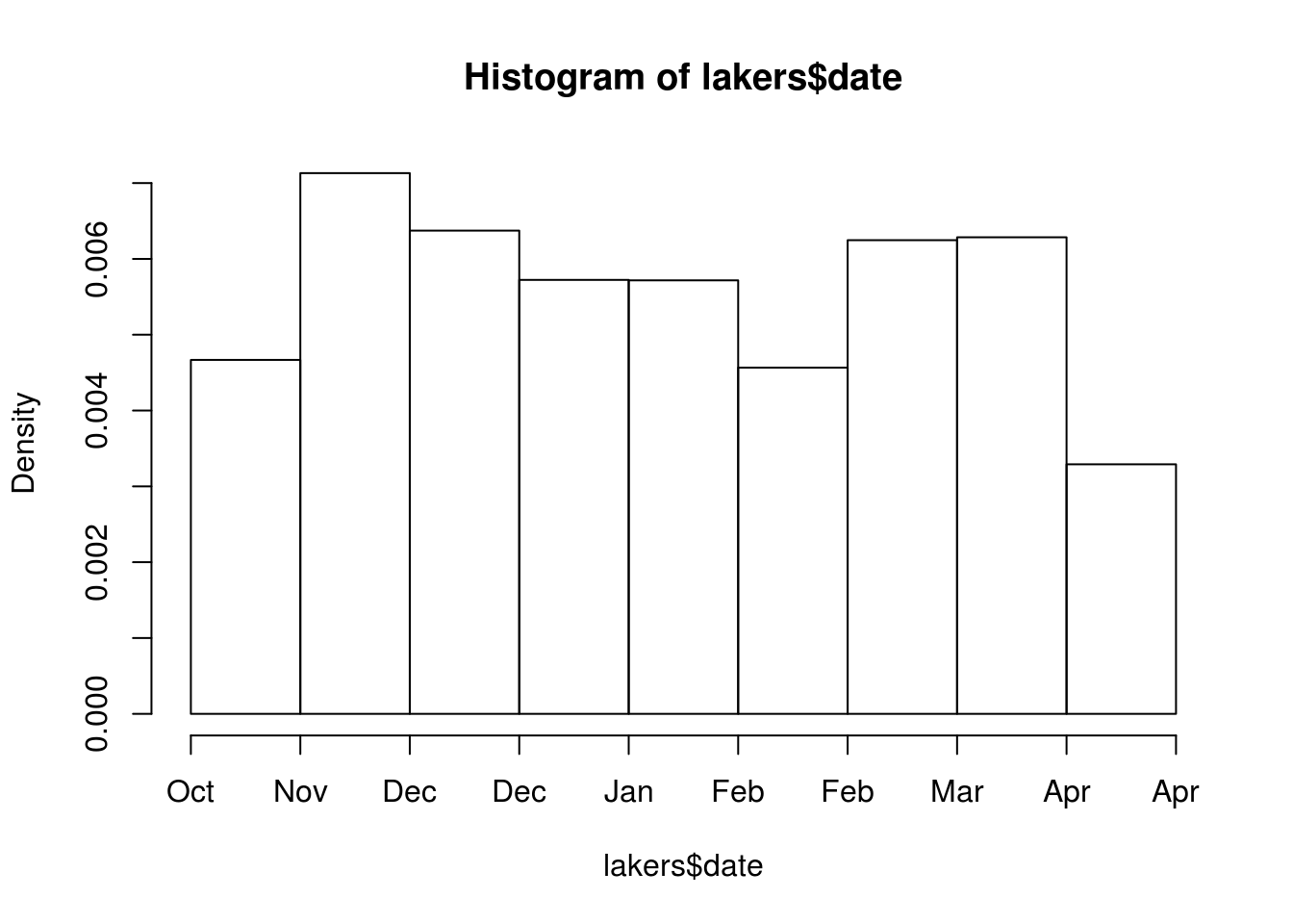
Time difference of 168 daysHowever, R does treat dates slightly differently from other numbers, and will format plot axes appropriately, which is helpful (see more on this in the graphics section):
hist(lakers$date, breaks=7)