25.1 Link functions

Logistic and poisson regression extend regular linear regression to allow us to constrain linear regression to predict within the rannge of possible outcomes. To achieve this, logistic regression, poisson regression and other members of the family of ‘generalised linear models’ use different ‘link functions’.

Link functions are used to connect the outcome variable to the linear model (that is, the linear combination of the parameters estimated for each of the predictors in the model). This means we can use linear models which still predict between -∞ and +∞, but without making inappropriate predictions.

For linear regression the link is simply the identity function — that is, the linear model directly predicts the outcome. However for other types of model different functions are used.

A good way to think about link functions is as a transformation of the model’s predictions. For example, in logistic regression predictions from the linear model are transformed in such a way that they are constrained to fall between 0 and 1. Thus, although to the underlying linear model allows values between -∞ and +∞, the link function ensures predictions fall between 0 and 1.

Logistic regression

When we have binary data, we want to be able run something like regression, but where we predict a probability of the outcome.

Because probabilities are limited to between 0 and 1, to link the data with the linear model we need to transform so they range from -∞ (infinity) to +∞.

You can think of the solution as coming in two steps:

Step 1

We can transform a probability on the 0—1 scale to a \(0 \rightarrow ∞\) scale by converting it to odds, which are expressed as a ratio:

\[odds = \dfrac{p}{1-p}\]

Probabilities and odds ratios are two equivalent ways of expressing the same idea.

So a probability of .5 equates to an odds ratio of 1 (i.e. 1 to 1); p=.6 equates to odds of 1.5 (that is, 1.5 to 1, or 3 to 2), and p = .95 equates to an odds ratio of 19 (19 to 1).

Odds convert or map probabilities from 0 to 1 onto the real numbers from 0 to ∞.

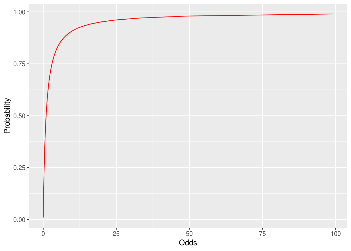
Figure 9.1: Probabilities converted to the odds scale. As p approaches 1 Odds goes to infinity.

We can reverse the transformation too (which is important later) because:

\[\textrm{probability} = \dfrac{\textrm{odds}}{1+\textrm{odds}}\]

• If a bookie gives odds of 66:1 on a horse, what probability does he think it has of winning?

• Why do bookies use odds and not probabilities?

• Should researchers use odds or probabilities when discussing with members of the public?

Step 2

When we convert a probability to odds, the odds will always be > zero.

This is still a problem for our linear model. We’d like our ‘regression’ coefficients to be able to vary between -∞ and ∞.

To avoid this restriction, we can take the logarithm of the odds — sometimes called the logit.

The figure below shows the transformation of probabilities between 0 and 1 to the log-odds scale. The logit has two nice properties:

1. It converts odds of less than one to negative numbers, because the log of a number between 0 and 1 is always negative[^1].

2. It flattens the rather square curve for the odds in the figure above, and

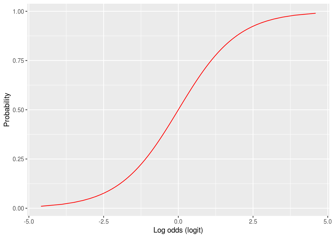
Figure 5.1: Probabilities converted to the logit (log-odds) scale. Notice how the slope implies that as probabilities approach 0 or 1 then the logit will get very large.

Reversing the process to interpret the model

As we’ve seen here, the logit or logistic link function transforms probabilities between 0/1 to the range from negative to positive infinity.

This means logistic regression coefficients are in log-odds units, so we must interpret logistic regression coefficients differently from regular regression with continuous outcomes.

• In linear regression, the coefficient is the change the outcome for a unit change in the predictor.

• For logistic regression, the coefficient is the change in the log odds of the outcome being 1, for a unit change in the predictor.

If we want to interpret logistic regression in terms of probabilities, we need to undo the transformation described in steps 1 and 2. To do this:

1. We take the exponent of the logit to ‘undo’ the log transformation. This gives us the predicted odds.

2. We convert the odds back to probability.

A hypothetical example

Imagine if we have a model to predict whether a person has any children. The outcome is binary, so equals 1 if the person has any children, and 0 otherwise.

The model has an intercept and one predictor, \(age\) in years. We estimate two parameters: \(\beta_0 = 0.5\) and \(\beta_{1} = 0.02\).

The outcome (\(y\)) of the linear model is the log-odds.

The model prediction is: \(\hat{y} = \beta_0 + \beta_1\textrm{age}\)

So, for someone aged 30:

• the predicted log-odds = \(0.5 + 0.02 * 30 = 1.1\)
• the predicted odds = \(exp(1.1) = 3.004\)
• the predicted probability = \(3.004 / (1 + 3.004) = .75\)

For someone aged 40:

• the predicted log-odds = \(0.5 + 0.02 * 40 = 1.3\)
• the predicted odds = \(exp(1.3) = 3.669\)
• the predicted probability = \(3.669 / (1 + 3.669) = .78\)

25.1.0.1 Regression coefficients are odds ratios

One final twist: In the section above we said that in logistic regression the coefficients are the change in the log odds of the outcome being 1, for a unit change in the predictor.

Without going into too much detail, one nice fact about logs is that if you take the log of two numbers and subtract them to take the difference, then this is equal to dividing the same numbers and then taking the log of the result:

A <- log(1)-log(5)
B  <- log(1/5)


# we have to use rounding because of limitations in
# the precision of R's arithmetic, but A and B are equal
round(A, 10) == round(B, 10)
[1] TRUE

This means that change in the log-odds is the same as the ratio of the odds

So, once we undo the log transformation by taking the exponent of the coefficient, we are left with the odds ratio.

You can now jump back to running logistic regression.