Pipes

We often want to combine select and filter (and other functions) to return a subset of our original data.

One way to achieve this is to ‘nest’ function calls.

Taking the mtcars data, we can select the weights of cars with a poor mpg:

gas.guzzlers <- select(filter(mtcars, mpg < 15), wt)
summary(gas.guzzlers)
       wt       
 Min.   :3.570  
 1st Qu.:3.840  
 Median :5.250  
 Mean   :4.686  
 3rd Qu.:5.345  
 Max.   :5.424  

This is OK, but can be confusing to read. The more deeply nested we go, the easier it is to make a mistake.

tidyverse provides an alternative to nested function calls, called the ‘pipe’.

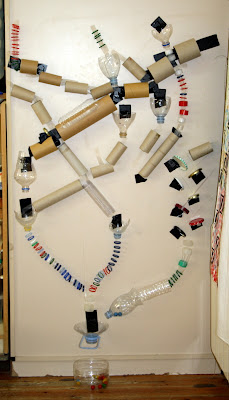
Imagine your dataframe as a big bucket, containing data.

From this bucket, you can ‘pour’ your data down the screen, and it passes through a series of tubes and filters.

At the bottom of your screen you have a smaller bucket, containing only the data you want.

Think of your data ‘flowing’ down the screen.

The ‘pipe’ operator, %>% makes our data ‘flow’ in this way:

big.bucket.of.data <- mtcars

big.bucket.of.data %>%
  filter(mpg <15) %>%
  select(wt) %>%
  summary
       wt       
 Min.   :3.570  
 1st Qu.:3.840  
 Median :5.250  
 Mean   :4.686  
 3rd Qu.:5.345  
 Max.   :5.424  

The %>% symbol makes the data flow onto the next step. Each function which follows the pipe takes the incoming data as it’s first input.

Pipes do the same thing as nesting functions, but the code stays more readable.

It’s especially nice because the order in which the functions happen is the same as the order in which we read the code (the opposite is true for nested functions).

We can save intermediate ‘buckets’ for use later on:

smaller.bucket <- big.bucket.of.data %>%
  filter(mpg <15) %>%
  select(wt)

This is an incredibly useful pattern for processing and working with data.

We can ‘pour’ data through a series of filters and other operations, saving intermediate states where necessary.

You can insert the %>% symbol in RStdudio by typing cmd-shift-M, which saves a lot of typing.