Checking assumptions

The text below continues on from this example of factorial Anova.

If we want to check that the assumptions of our Anova models are met, these tables and plots would be a reasonable place to start. First running Levene’s test:

car::leveneTest(eysenck.model) %>%
  pander()

Levene’s Test for Homogeneity of Variance (center = median)

	Df	F value	Pr(>F)
group	9	1.031	0.4217
	90	NA	NA

Then a QQ-plot of the model residuals to assess normality:

car::qqPlot(eysenck.model)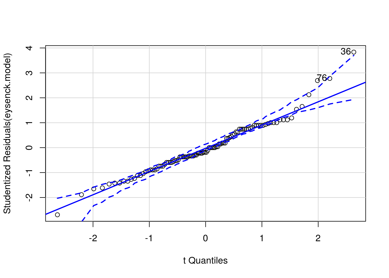

Figure 8.1: QQ plot to assess normality of model residuals

[1] 36 76

And finally a residual-vs-fitted plot:

data_frame(
  fitted = predict(eysenck.model),
  residual = residuals(eysenck.model)) %>%
  # and then plot points and a smoothed line
  ggplot(aes(fitted, residual)) +
    geom_point() +
    geom_smooth(se=F)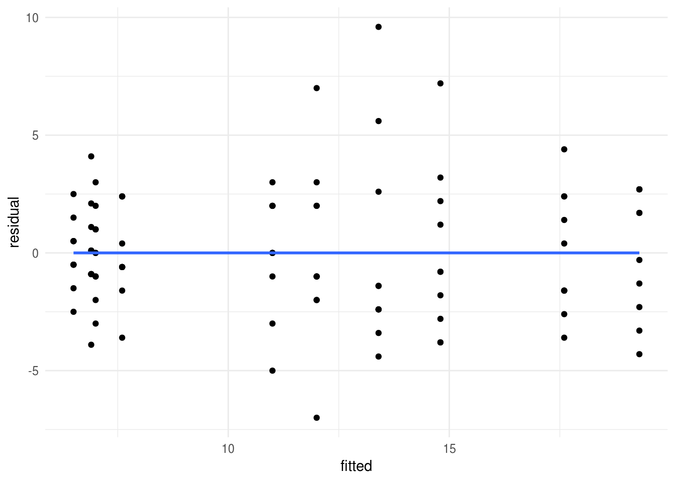

Figure 8.2: Residual vs fitted (spread vs. level) plot to check homogeneity of variance.

For more on assumptions checks after linear models or Anova see: http://www.statmethods.net/stats/anovaAssumptions.html