12 Baysian model fitting
Baysian fitting of linear models via MCMC methods
This is a minimal guide to fitting and interpreting regression and multilevel models via MCMC. For much more detail, and a much more comprehensive introduction to modern Bayesian analysis see Jon Kruschke’s Doing Bayesian Data Analysis.
Let’s revisit our previous example which investigated the effect of familiar and liked music on pain perception:
painmusic <- readRDS('data/painmusic.RDS')
painmusic %>%
  ggplot(aes(liked, with.music - no.music,
             group=familiar, color=familiar)) +
  stat_summary(geom="pointrange", fun.data=mean_se) +
  stat_summary(geom="line",  fun.data=mean_se) +
  ylab("Pain (VAS) with.music - no.music") +
  scale_color_discrete(name="") +
  xlab("")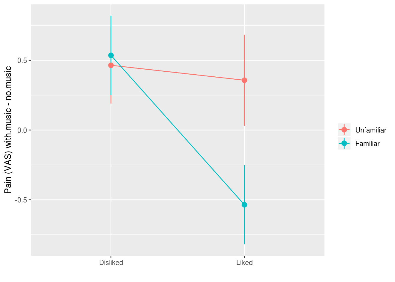
# set sum contrasts
options(contrasts = c("contr.sum", "contr.poly"))
pain.model <- lm(with.music ~
                   no.music + familiar * liked,
                 data=painmusic)
summary(pain.model)

Call:
lm(formula = with.music ~ no.music + familiar * liked, data = painmusic)

Residuals:
    Min      1Q  Median      3Q     Max
-3.5397 -1.0123 -0.0048  0.9673  4.8882

Coefficients:
                 Estimate Std. Error t value Pr(>|t|)
(Intercept)       1.55899    0.40126   3.885 0.000177 ***
no.music          0.73588    0.07345  10.019  < 2e-16 ***
familiar1         0.20536    0.13895   1.478 0.142354
liked1            0.30879    0.13900   2.222 0.028423 *
familiar1:liked1 -0.18447    0.13983  -1.319 0.189909
---
Signif. codes:  0 '***' 0.001 '**' 0.01 '*' 0.05 '.' 0.1 ' ' 1

Residual standard error: 1.47 on 107 degrees of freedom
Multiple R-squared:  0.5043,    Adjusted R-squared:  0.4858
F-statistic: 27.22 on 4 and 107 DF,  p-value: 1.378e-15
Do the same thing again, but with with MCMC using Stan:
library(rstanarm)
options(contrasts = c("contr.sum", "contr.poly"))
pain.model.mcmc <- stan_lm(with.music ~ no.music + familiar * liked,
data=painmusic, prior=NULL)summary(pain.model.mcmc)
Model Info:
function: stan_lm
family: gaussian [identity]
formula: with.music ~ no.music + familiar * liked
algorithm: sampling
priors: see help('prior_summary')
sample: 4000 (posterior sample size)
observations: 112
predictors: 5
Estimates:
mean sd 2.5% 25% 50% 75% 97.5%
(Intercept) 1.7 0.4 0.9 1.4 1.7 2.0 2.5
no.music 0.7 0.1 0.6 0.7 0.7 0.8 0.9
familiar1 0.2 0.1 -0.1 0.1 0.2 0.3 0.5
liked1 0.3 0.1 0.0 0.2 0.3 0.4 0.6
familiar1:liked1 -0.2 0.1 -0.5 -0.3 -0.2 -0.1 0.1
sigma 1.5 0.1 1.3 1.4 1.5 1.5 1.7
log-fit_ratio 0.0 0.1 -0.1 0.0 0.0 0.0 0.1
R2 0.5 0.1 0.3 0.4 0.5 0.5 0.6
mean_PPD 5.3 0.2 4.9 5.2 5.3 5.5 5.7
log-posterior -206.1 2.3 -211.9 -207.3 -205.8 -204.5 -202.6
Diagnostics:
mcse Rhat n_eff
(Intercept) 0.0 1.0 1389
no.music 0.0 1.0 1371
familiar1 0.0 1.0 3272
liked1 0.0 1.0 4350
familiar1:liked1 0.0 1.0 3624
sigma 0.0 1.0 3902
log-fit_ratio 0.0 1.0 1971
R2 0.0 1.0 1672
mean_PPD 0.0 1.0 4225
log-posterior 0.1 1.0 927
For each parameter, mcse is Monte Carlo standard error, n_eff is a crude measure of effective sample size, and Rhat is the potential scale reduction factor on split chains (at convergence Rhat=1).Posterior probabilities for parameters
library(bayesplot)

mcmc_areas(as.matrix(pain.model.mcmc), regex_pars = 'familiar|liked', prob = .9)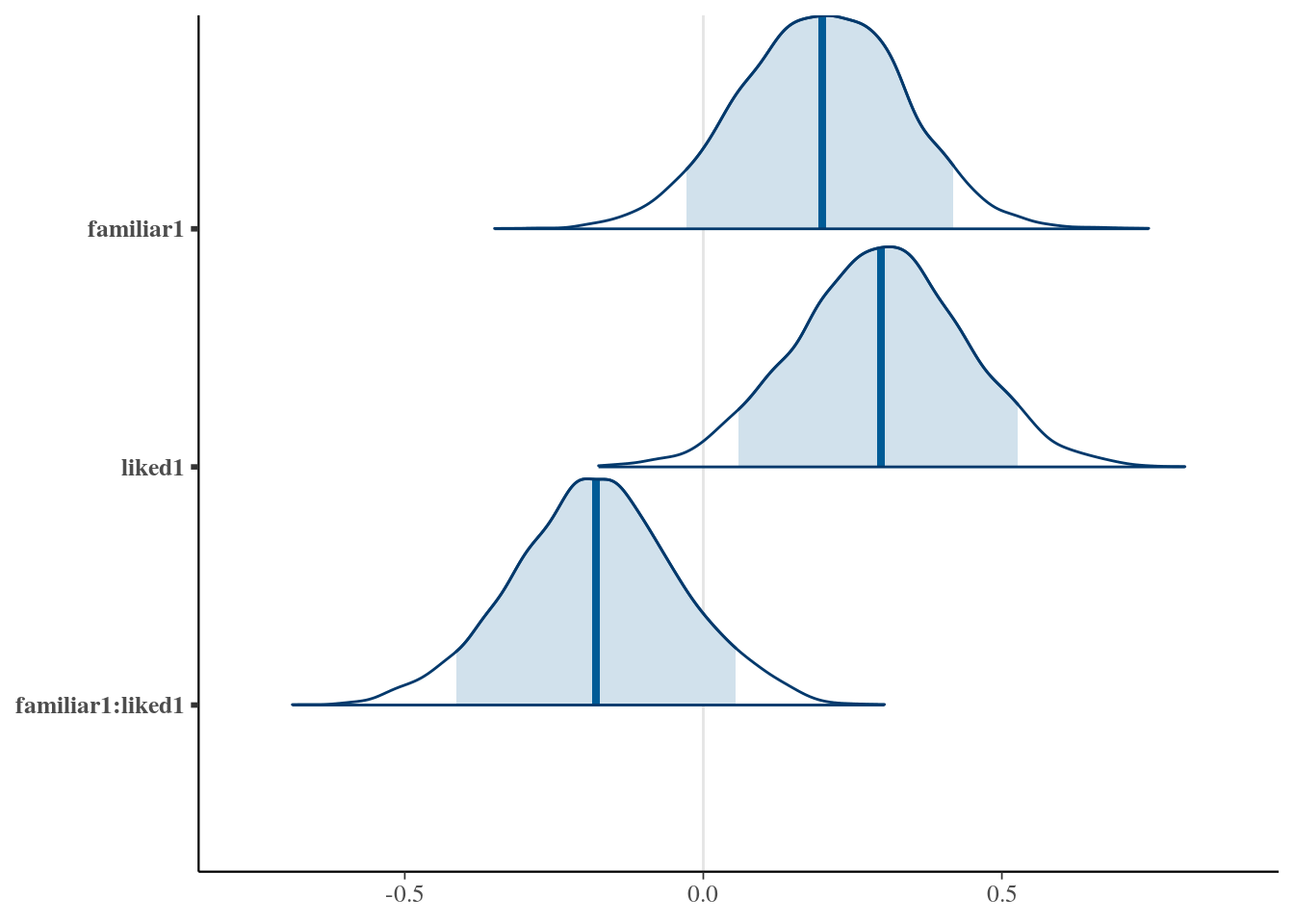
mcmc_intervals(as.matrix(pain.model.mcmc), regex_pars = 'familiar|liked', prob_outer = .9)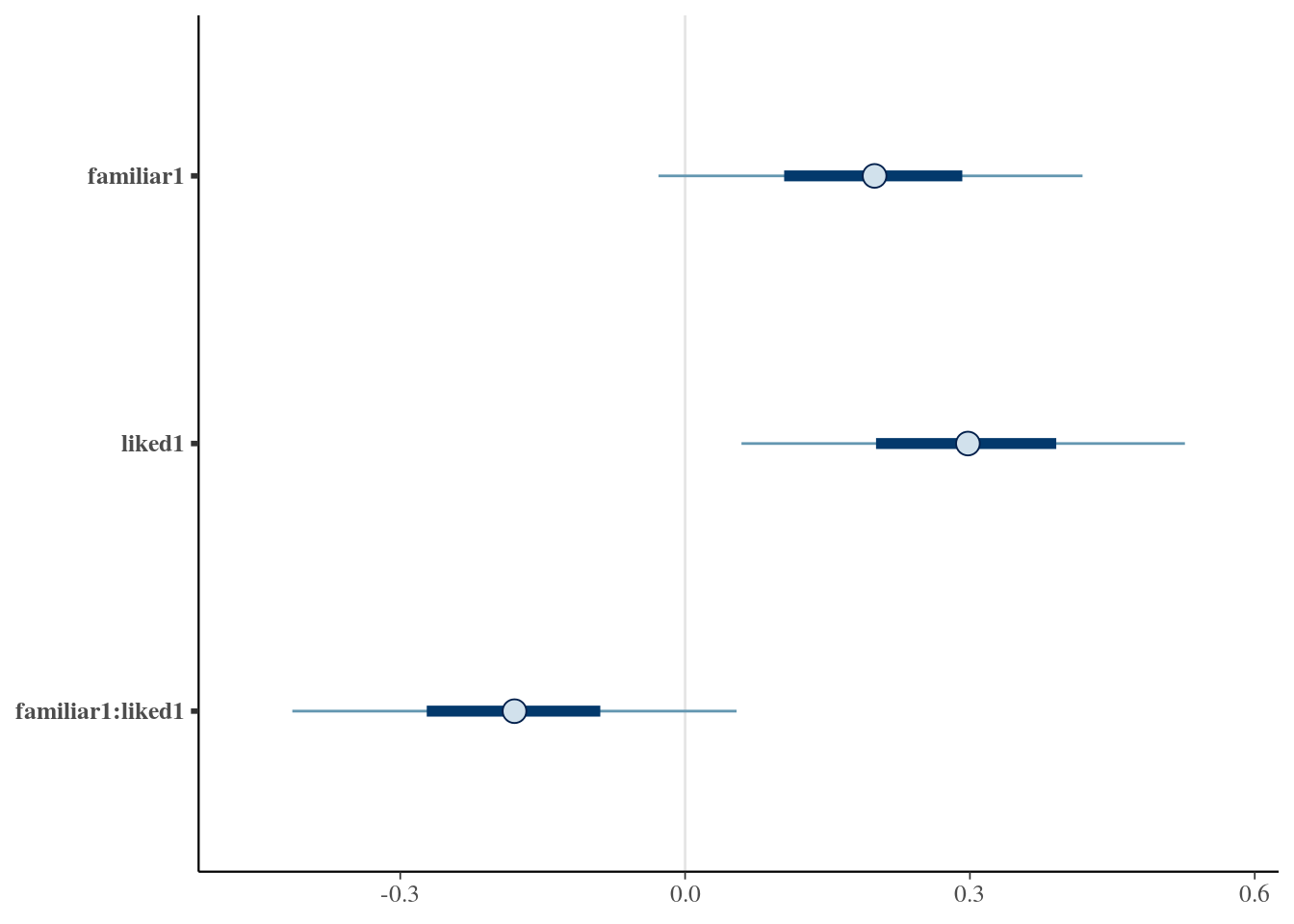
Credible intervals
Credible intervals are distinct from confidence intervals
TODO EXPAND
params.of.interest <-
  pain.model.mcmc %>%
  as_tibble %>%
  reshape2::melt() %>%
  filter(stringr::str_detect(variable, "famil|liked")) %>%
  group_by(variable)

params.of.interest %>%
  tidybayes::mean_hdi() %>%
  pander::pandoc.table(caption="Estimates and 95% credible intervals for the parameters of interest")

------------------------------------------------------------------------------
     variable        value     .lower    .upper   .width   .point   .interval
------------------ --------- ---------- -------- -------- -------- -----------
    familiar1       0.1979    -0.06647   0.4635    0.95     mean       hdi

      liked1        0.2963    0.01164    0.5591    0.95     mean       hdi

 familiar1:liked1   -0.1798   -0.4437    0.1075    0.95     mean       hdi
------------------------------------------------------------------------------

Table: Estimates and 95% credible intervals for the parameters of interest
Bayesian ‘p values’ for parameters
We can do simple arithmetic with the posterior draws to calculate the probability a parameter is greater than (or less than) zero:
params.of.interest %>%
  summarise(estimate=mean(value),
            `p (x<0)` = mean(value < 0),
            `p (x>0)` = mean(value > 0))
# A tibble: 3 x 4
  variable         estimate `p (x<0)` `p (x>0)`
  <fct>               <dbl>     <dbl>     <dbl>
1 familiar1           0.198    0.0742     0.926
2 liked1              0.296    0.0182     0.982
3 familiar1:liked1   -0.180    0.899      0.101
Or if you’d like the Bayes Factor (evidence ratio) for one hypotheses vs
another, for example comparing the hypotheses that a parameter is > vs. <= 0,
then you can use the hypothesis function in the brms package:
pain.model.mcmc.df <-
  pain.model.mcmc %>%
  as_tibble

brms::hypothesis(pain.model.mcmc.df,
                 c("familiar1 > 0",
                   "liked1 > 0",
                   "familiar1:liked1 < 0"))
Hypothesis Tests for class :
              Hypothesis Estimate Est.Error CI.Lower CI.Upper Evid.Ratio
1        (familiar1) > 0     0.20      0.14    -0.03      Inf      12.47
2           (liked1) > 0     0.30      0.14     0.06      Inf      53.79
3 (familiar1:liked1) < 0    -0.18      0.14     -Inf     0.05       8.88
  Post.Prob Star
1      0.93
2      0.98    *
3      0.90
---
'*': The expected value under the hypothesis lies outside the 95%-CI.
Posterior probabilities of point hypotheses assume equal prior probabilities.
Here although we only have a ‘significant’ p value for one of the parameters, we can also see there is “very strong” evidence that familiarity also influences pain, and “strong” evidence for the interaction of familiarity and liking, according to conventional rules of thumb when interpreting Bayes Factors.
TODO - add a fuller explanation of why multiple comparisons are not an issue for Bayesian analysis [@gelman2012we], because p values do not have the same interpretation in terms of long run frequencies of replication; they are a representation of the weight of the evidence in favour of a hypothesis.
TODO: Also reference Zoltan Dienes Bayes paper.