Extending traditional RM Anova

As noted in the Anova cookbook section, repeated measures anova can be approximated using linear mixed models.

For example, reprising the sleepstudy example, we can approximate a repeated measures Anova in which multiple measurements of Reaction time are taken on multiple Days for each Subject.

As we saw before, the traditional RM Anova model is:

sleep.rmanova <- afex::aov_car(Reaction ~ Days + Error(Subject/(Days)), data=lme4::sleepstudy)
Registered S3 methods overwritten by 'car':
  method                          from
  influence.merMod                lme4
  cooks.distance.influence.merMod lme4
  dfbeta.influence.merMod         lme4
  dfbetas.influence.merMod        lme4
sleep.rmanova
Anova Table (Type 3 tests)

Response: Reaction
  Effect          df     MSE         F ges p.value
1   Days 3.32, 56.46 2676.18 18.70 *** .29  <.0001
---
Signif. codes:  0 '***' 0.001 '**' 0.01 '*' 0.05 '+' 0.1 ' ' 1

Sphericity correction method: GG 

The equivalent lmer model is:

library(lmerTest)
sleep.lmer <- lmer(Reaction ~ factor(Days) + (1|Subject), data=lme4::sleepstudy)
anova(sleep.lmer)
Type III Analysis of Variance Table with Satterthwaite's method
             Sum Sq Mean Sq NumDF DenDF F value    Pr(>F)    
factor(Days) 166235   18471     9   153  18.703 < 2.2e-16 ***
---
Signif. codes:  0 '***' 0.001 '**' 0.01 '*' 0.05 '.' 0.1 ' ' 1

The following sections demonstrate just some of the extensions to RM Anova which are possible with mutlilevel models,

Fit a simple slope for Days

lme4::sleepstudy %>%
  ggplot(aes(Days, Reaction)) +
  geom_point() + geom_jitter() +
  geom_smooth()
`geom_smooth()` using method = 'loess' and formula 'y ~ x'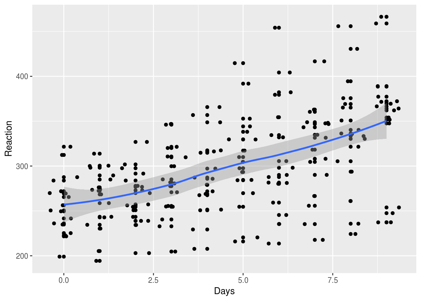

slope.model <- lmer(Reaction ~ Days + (1|Subject),  data=lme4::sleepstudy)
anova(slope.model)
Type III Analysis of Variance Table with Satterthwaite's method
     Sum Sq Mean Sq NumDF DenDF F value    Pr(>F)    
Days 162703  162703     1   161   169.4 < 2.2e-16 ***
---
Signif. codes:  0 '***' 0.001 '**' 0.01 '*' 0.05 '.' 0.1 ' ' 1
slope.model.summary <- summary(slope.model)
slope.model.summary$coefficients
             Estimate Std. Error       df  t value     Pr(>|t|)
(Intercept) 251.40510  9.7467163  22.8102 25.79383 2.241351e-18
Days         10.46729  0.8042214 161.0000 13.01543 6.412601e-27

Allow the effect of sleep deprivation to vary for different participants

If we plot the data, it looks like sleep deprivation hits some participants worse than others:

set.seed(1234)
lme4::sleepstudy %>%
  filter(Subject %in% sample(levels(Subject), 10)) %>%
  ggplot(aes(Days, Reaction, group=Subject, color=Subject)) +
  geom_smooth(method="lm", se=F) +
  geom_jitter(size=1) +
  theme_minimal()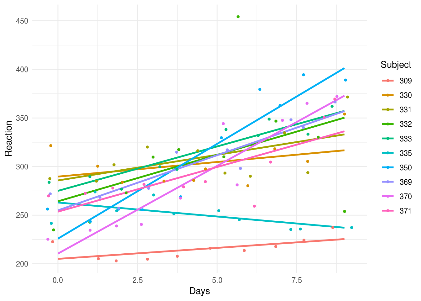

If we wanted to test whether there was significant variation in the effects of sleep deprivation between subjects, by adding a random slope to the model.

The random slope allows the effect of Days to vary between subjects. So we can think of an overall slope (i.e. RT goes up over the days), from which individuals deviate by some amount (e.g. a resiliant person will have a negative deviation or residual from the overall slope).

Adding the random slope doesn’t change the F test for Days that much:

random.slope.model <- lmer(Reaction ~ Days + (Days|Subject),  data=lme4::sleepstudy)
anova(random.slope.model)
Type III Analysis of Variance Table with Satterthwaite's method
     Sum Sq Mean Sq NumDF  DenDF F value    Pr(>F)    
Days  30024   30024     1 16.995  45.843 3.273e-06 ***
---
Signif. codes:  0 '***' 0.001 '**' 0.01 '*' 0.05 '.' 0.1 ' ' 1

Nor the overall slope coefficient:

random.slope.model.summary <- summary(random.slope.model)
slope.model.summary$coefficients
             Estimate Std. Error       df  t value     Pr(>|t|)
(Intercept) 251.40510  9.7467163  22.8102 25.79383 2.241351e-18
Days         10.46729  0.8042214 161.0000 13.01543 6.412601e-27

But we can use the lmerTest::ranova() function to show that there is statistically significant variation in slopes between individuals, using the likelihood ratio test:

lmerTest::ranova(random.slope.model)
ANOVA-like table for random-effects: Single term deletions

Model:
Reaction ~ Days + (Days | Subject)
                         npar  logLik    AIC    LRT Df Pr(>Chisq)    
<none>                      6 -871.81 1755.6                         
Days in (Days | Subject)    4 -893.23 1794.5 42.837  2   4.99e-10 ***
---
Signif. codes:  0 '***' 0.001 '**' 0.01 '*' 0.05 '.' 0.1 ' ' 1

Because the random slope for Days is statistically significant, we know it improves the model. One way to see that improvement is to plot residuals (unexplained error for each datapoint) against predicted values. To extract residual and fitted values we use the residuals() and predict() functions. These are then combined in a data_frame, to enable us to use ggplot for the subsequent figures.

# create data frames containing residuals and fitted
# values for each model we ran above
a <-  data_frame(
    model = "random.slope",
    fitted = predict(random.slope.model),
    residual = residuals(random.slope.model))
Warning: `data_frame()` is deprecated, use `tibble()`.
This warning is displayed once per session.
b <- data_frame(
    model = "random.intercept",
    fitted = predict(slope.model),
    residual = residuals(slope.model))

# join the two data frames together
residual.fitted.data <- bind_rows(a,b)

We can see that the residuals from the random slope model are much more evenly distributed across the range of fitted values, which suggests that the assumption of homogeneity of variance is met in the random slope model:

# plots residuals against fitted values for each model
residual.fitted.data %>%
  ggplot(aes(fitted, residual)) +
  geom_point() +
  geom_smooth(se=F) +
  facet_wrap(~model)
`geom_smooth()` using method = 'loess' and formula 'y ~ x'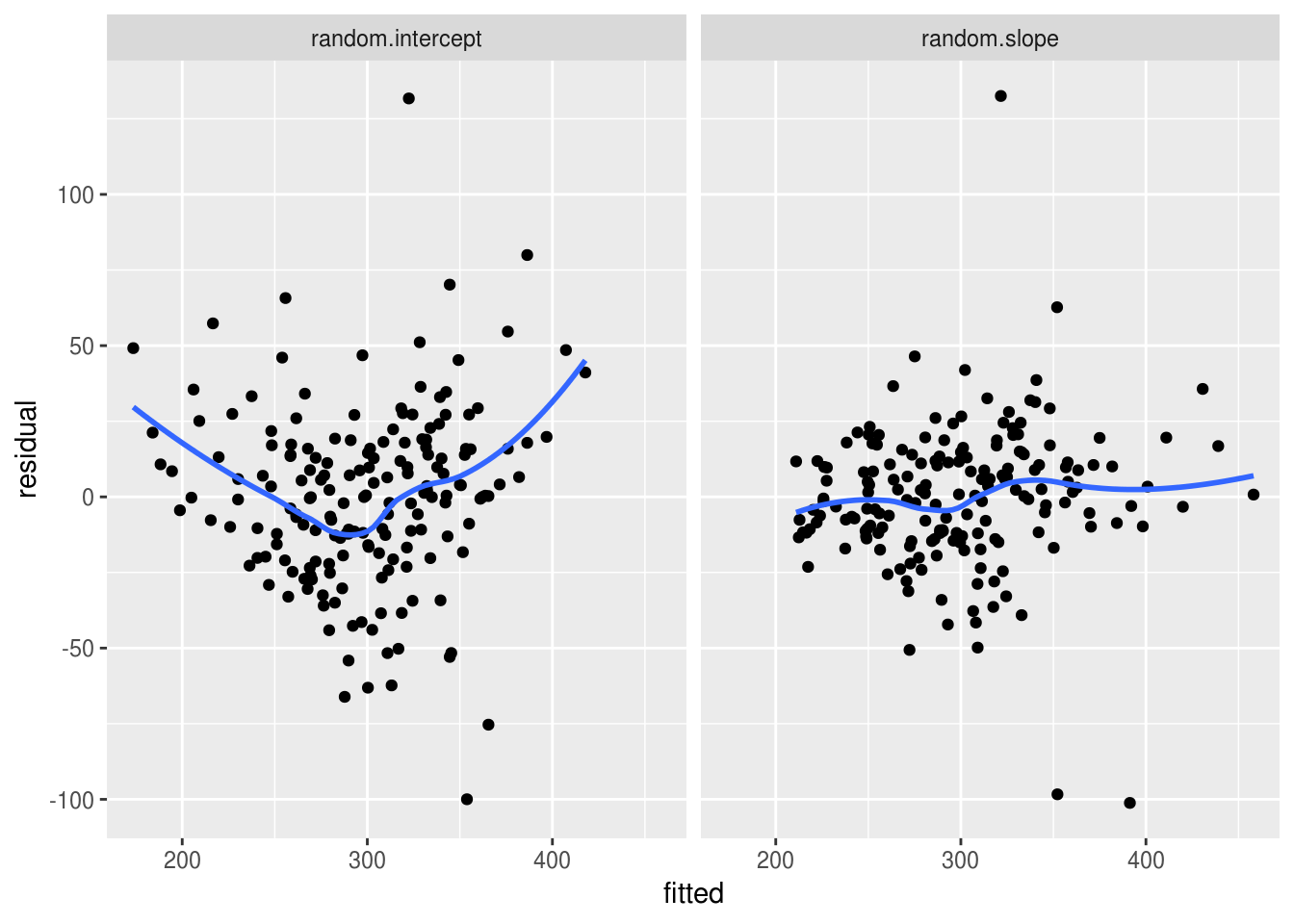

We can plot both of the random effects from this model (intercept and slope) to see how much the model expects individuals to deviate from the overall (mean) slope.

# extract the random effects from the model (intercept and slope)
ranef(random.slope.model)$Subject %>%
  # implicitly convert them to a dataframe and add a column with the subject number
  rownames_to_column(var="Subject") %>%
  # plot the intercept and slobe values with geom_abline()
  ggplot(aes()) +
  geom_abline(aes(intercept=`(Intercept)`, slope=Days, color=Subject)) +
  # add axis label
  xlab("Day") + ylab("Residual RT") +
  # set the scale of the plot to something sensible
  scale_x_continuous(limits=c(0,10), expand=c(0,0)) +
  scale_y_continuous(limits=c(-100, 100))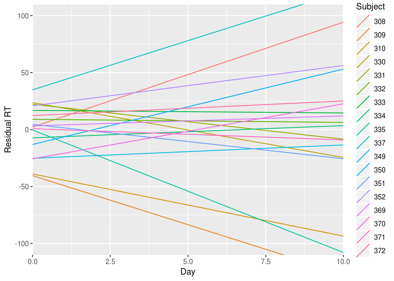

Inspecting this plot, there doesn’t seem to be any strong correlation between the RT value at which an individual starts (their intercept residual) and the slope describing how they change over the days compared with the average slope (their slope residual).

That is, we can’t say that knowing whether a person has fast or slow RTs at the start of the study gives us a clue about what will happen to them after they are sleep deprived: some people start slow and get faster; other start fast but suffer and get slower.

However we can explicitly check this correlation (between individuals’ intercept and slope residuals) using the VarCorr() function:

VarCorr(random.slope.model)
 Groups   Name        Std.Dev. Corr 
 Subject  (Intercept) 24.7366       
          Days         5.9229  0.066
 Residual             25.5918       

The correlation between the random intercept and slopes is only 0.066, and so very low. We might, therefore, want to try fitting a model without this correlation. lmer includes the correlation by default, so we need to change the model formula to make it clear we don’t want it:

uncorrelated.reffs.model <- lmer(
  Reaction ~ Days + (1 | Subject) + (0 + Days|Subject),
  data=lme4::sleepstudy)

VarCorr(uncorrelated.reffs.model)
 Groups    Name        Std.Dev.
 Subject   (Intercept) 25.0499 
 Subject.1 Days         5.9887 
 Residual              25.5652 

The variance components don’t change much when we constrain the covariance of intercepts and slopes to be zero, and we can explicitly compare these two models using the anova() function, which is somewhat confusingly named because in this instance it is performing a likelihood ratio test to compare the two models:

anova(random.slope.model, uncorrelated.reffs.model)
refitting model(s) with ML (instead of REML)
Data: lme4::sleepstudy
Models:
uncorrelated.reffs.model: Reaction ~ Days + (1 | Subject) + (0 + Days | Subject)
random.slope.model: Reaction ~ Days + (Days | Subject)
                         Df    AIC    BIC  logLik deviance  Chisq Chi Df
uncorrelated.reffs.model  5 1762.0 1778.0 -876.00   1752.0              
random.slope.model        6 1763.9 1783.1 -875.97   1751.9 0.0639      1
                         Pr(>Chisq)
uncorrelated.reffs.model           
random.slope.model           0.8004

Model fit is not significantly worse with the constrained model, so for parsimony’s sake we prefer it to the more complex model.

Fitting a curve for the effect of Days

In theory, we could also fit additional parameters for the effect of Days, although a combined smoothed line plot/scatterplot indicates that a linear function fits the data reasonably well.

lme4::sleepstudy %>%
  ggplot(aes(Days, Reaction)) +
  geom_point() + geom_jitter() +
  geom_smooth()
`geom_smooth()` using method = 'loess' and formula 'y ~ x'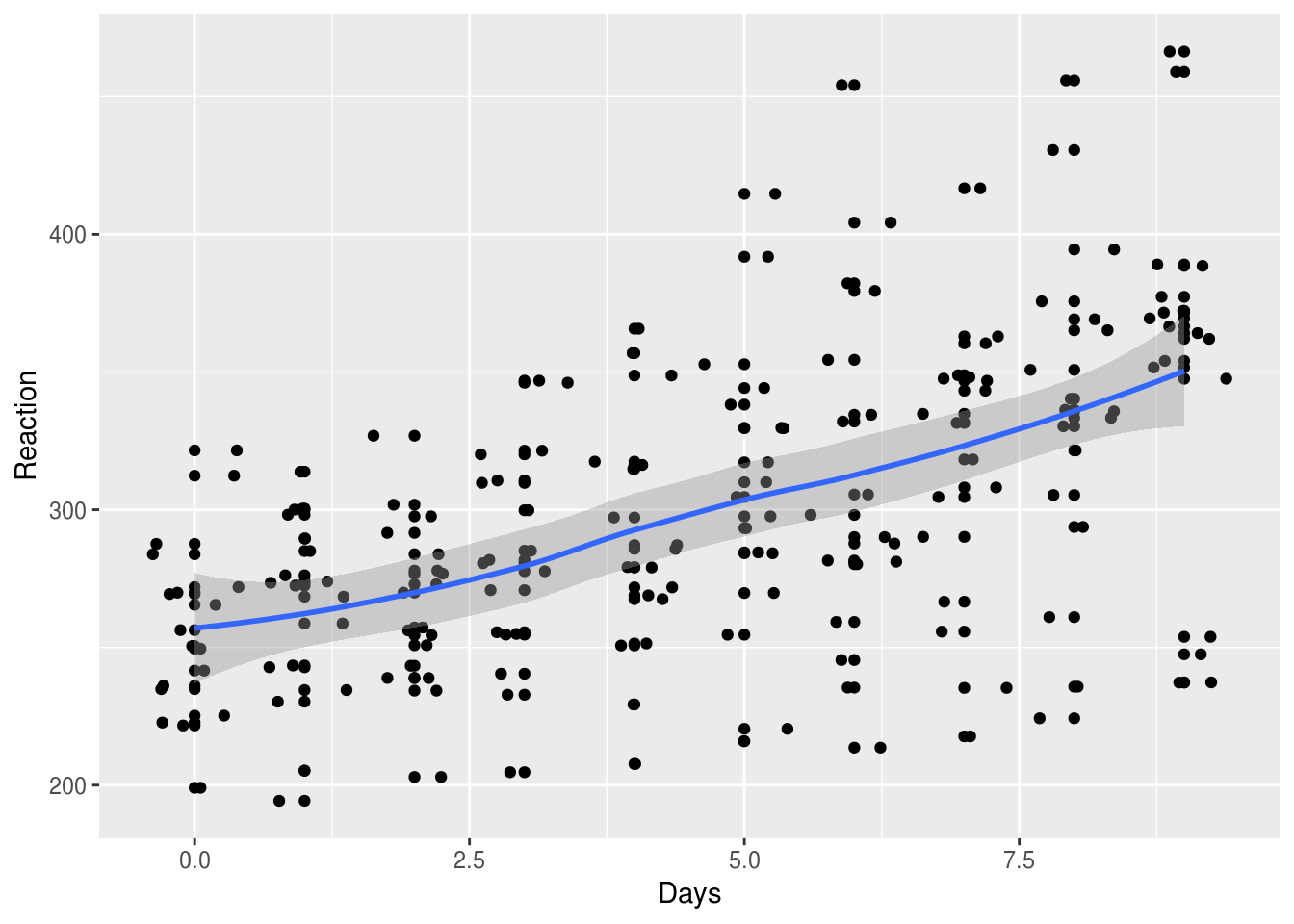

If we insisted on testing a curved (quadratic) function of Days, we could:

quad.model <- lmer(Reaction ~ Days + I(Days^2) + (1|Subject),  data=lme4::sleepstudy)
quad.model.summary <- summary(quad.model)
quad.model.summary$coefficients
               Estimate Std. Error        df   t value     Pr(>|t|)
(Intercept) 255.4493728 10.4656347  30.04058 24.408398 2.299848e-21
Days          7.4340850  2.9707976 160.00001  2.502387 1.334036e-02
I(Days^2)     0.3370223  0.3177733 160.00001  1.060575 2.904815e-01

Here, the p value for I(Days^2) is not significant, suggesting (as does the plot) that a simple slope model is sufficient.