Confirmatory factor analysis (CFA)
In psychology we make observations, but we’re often interested in hypothetical constructs, e.g. Anxiety, working memory. We can’t measure these directly, but we assume that our observations are related to these constructs in some way.
Regression and related techniques (e.g. Anova) require us to assume that our outcome variables are good indices of these underlying constructs, and that our predictor variables are measured without any error.
When outcomes are straightforward observed variables like plant yield or weight reduction, and where predictors are experimentally manipulated, then these assumptions are reasonable. However in many applied fields these are not reasonable assumptions to make: For example, to assume that depression or working memory are indexed in a straightforward way by responses to a depression questionnaire or performance on a laboratory task is naive. Likewise, we should not assume that a construct like working memory is measured without error when we use it to predict some other outcome (e.g. exam success).
Confirmatory factor analysis (CFA), structural equation models (SEM) and related techniques are designed to help researchers deal with these imperfections in our observations, and can help to explore the correspondence between our measures and the underlying constructs of interest.
Latent variables
CFA and SEM introduce the concept of a latent variable which is either the cause of, or formed by, the observations we make. Latent variables aren’t quite the same thing as hypothetical constructs, but they are similar many in some ways. The original distinction between hypothetical constructs and intervening variables is quite interesting in this context, see Maccorquodale and Meehl (1948).
To achieve this, CFA requires that researchers to make predictions about the patterns of correlations they will observe in their observations, based on the process they think is generating the data. CFA provides a mechanism to test and compare different hypotheses about these patterns, which correspond to different models of the underlying process which generates the data.
It is conventional within CFA and SEM to extend the graphical models used to describe path models (see above). In these diagrams, square edged boxes represent observed variables, and rounded or oval boxes represent latent variables, sometimes called factors:
knit_gv('
Factor -> a
Factor -> b
Factor -> c
Factor -> d
a[shape=rectangle]
b[shape=rectangle]
c[shape=rectangle]
d[shape=rectangle]
')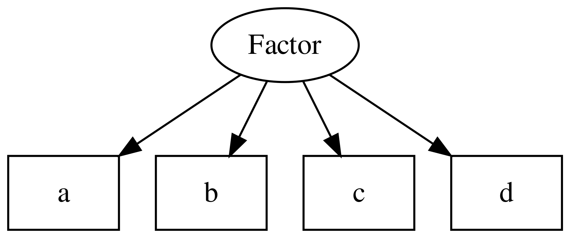
Figure 10.1: Example of a CFA model, including one latent variable or factor, and 4 observed variables.
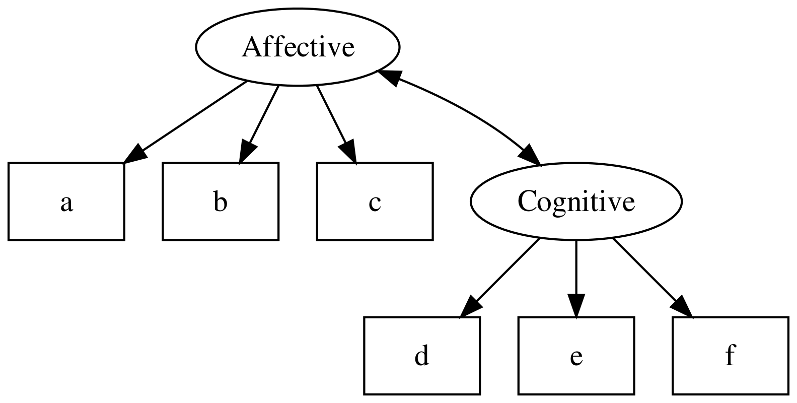
CFA models can also include multiple latent variables, and estimate the covariance between them:
knit_gv('
        Affective -> a
Affective -> b
Affective -> c
Cognitive -> d
Cognitive -> e
Cognitive -> f
Affective -> Cognitive:nw [dir=both]

a [shape=box]
b [shape=box]
c [shape=box]
d [shape=box]
e [shape=box]
f [shape=box]

')
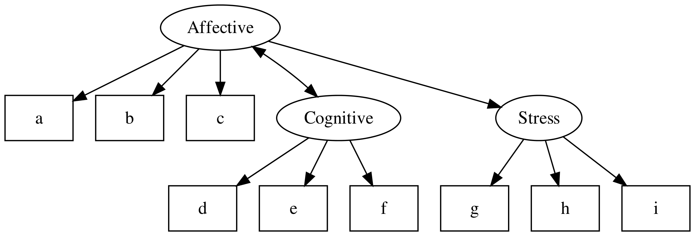
SEM models extend this by allowing regression paths between latent variables and observed or other latent variables:
knit_gv('
        Affective -> a
Affective -> b
Affective -> c
Cognitive -> d
Cognitive -> e
Cognitive -> f
Affective -> Cognitive:nw [dir=both]

a [shape=box]
b [shape=box]
c [shape=box]
d [shape=box]
e [shape=box]
f [shape=box]


Stress -> g
Stress -> h
Stress -> i
g [shape=box]
h [shape=box]
i [shape=box]

Affective -> Stress

        ')
For now though, we will focus on building a CFA model. Later we’ll show how a well fitting measurement model can be used to test hypotheses related to the structural relations between latent variables.
Defining a CFA model
First, open some data and check that all looks well. This is a classic CFA example — see the help file for more info.
hz <- lavaan::HolzingerSwineford1939
hz %>% glimpse()
Observations: 301
Variables: 15
$ id     <int> 1, 2, 3, 4, 5, 6, 7, 8, 9, 11, 12, 13, 14, 15, 16, 17, 18…
$ sex    <int> 1, 2, 2, 1, 2, 2, 1, 2, 2, 2, 1, 1, 2, 2, 1, 2, 2, 1, 2, …
$ ageyr  <int> 13, 13, 13, 13, 12, 14, 12, 12, 13, 12, 12, 12, 12, 12, 1…
$ agemo  <int> 1, 7, 1, 2, 2, 1, 1, 2, 0, 5, 2, 11, 7, 8, 6, 1, 11, 5, 8…
$ school <fct> Pasteur, Pasteur, Pasteur, Pasteur, Pasteur, Pasteur, Pas…
$ grade  <int> 7, 7, 7, 7, 7, 7, 7, 7, 7, 7, 7, 7, 7, 7, 7, 7, 7, 7, 7, …
$ x1     <dbl> 3.333333, 5.333333, 4.500000, 5.333333, 4.833333, 5.33333…
$ x2     <dbl> 7.75, 5.25, 5.25, 7.75, 4.75, 5.00, 6.00, 6.25, 5.75, 5.2…
$ x3     <dbl> 0.375, 2.125, 1.875, 3.000, 0.875, 2.250, 1.000, 1.875, 1…
$ x4     <dbl> 2.333333, 1.666667, 1.000000, 2.666667, 2.666667, 1.00000…
$ x5     <dbl> 5.75, 3.00, 1.75, 4.50, 4.00, 3.00, 6.00, 4.25, 5.75, 5.0…
$ x6     <dbl> 1.2857143, 1.2857143, 0.4285714, 2.4285714, 2.5714286, 0.…
$ x7     <dbl> 3.391304, 3.782609, 3.260870, 3.000000, 3.695652, 4.34782…
$ x8     <dbl> 5.75, 6.25, 3.90, 5.30, 6.30, 6.65, 6.20, 5.15, 4.65, 4.5…
$ x9     <dbl> 6.361111, 7.916667, 4.416667, 4.861111, 5.916667, 7.50000…
As noted above, to define models in lavaan you must specify the relationships
between variables in a text format. A full
guide to this lavaan model syntax is available on the project website.
For CFA models, like path models, the format is fairly simple, and resembles a series of linear models, written over several lines.
In the model below there are three latent variables, visual, writing and
maths. The latent variable names are followed by =~ which means ‘is manifested
by’, and then the observed variables, our measures for the latent variable, are
listed, separated by the + symbol.
hz.model <- '
visual =~ x1 + x2 + x3
writing =~ x4 + x5 + x6
maths =~ x7 + x8 + x9'
Note that we have saved our model specification/syntax in a variable named
hz.model.
The other special symbols in the lavaan syntax which can be used for CFA
models are:
a ~~ b, which represents a covariance.a ~~ a, which is a variance (you can think of this as the covariance of a variable with itself)
To run the analysis we again pass the model specification and the data to the
cfa() function:
hz.fit <- cfa(hz.model, data=hz)
summary(hz.fit, standardized=TRUE)
lavaan 0.6-3 ended normally after 35 iterations

  Optimization method                           NLMINB
  Number of free parameters                         21

  Number of observations                           301

  Estimator                                         ML
  Model Fit Test Statistic                      85.306
  Degrees of freedom                                24
  P-value (Chi-square)                           0.000

Parameter Estimates:

  Information                                 Expected
  Information saturated (h1) model          Structured
  Standard Errors                             Standard

Latent Variables:
                   Estimate  Std.Err  z-value  P(>|z|)   Std.lv  Std.all
  visual =~
    x1                1.000                               0.900    0.772
    x2                0.554    0.100    5.554    0.000    0.498    0.424
    x3                0.729    0.109    6.685    0.000    0.656    0.581
  writing =~
    x4                1.000                               0.990    0.852
    x5                1.113    0.065   17.014    0.000    1.102    0.855
    x6                0.926    0.055   16.703    0.000    0.917    0.838
  maths =~
    x7                1.000                               0.619    0.570
    x8                1.180    0.165    7.152    0.000    0.731    0.723
    x9                1.082    0.151    7.155    0.000    0.670    0.665

Covariances:
                   Estimate  Std.Err  z-value  P(>|z|)   Std.lv  Std.all
  visual ~~
    writing           0.408    0.074    5.552    0.000    0.459    0.459
    maths             0.262    0.056    4.660    0.000    0.471    0.471
  writing ~~
    maths             0.173    0.049    3.518    0.000    0.283    0.283

Variances:
                   Estimate  Std.Err  z-value  P(>|z|)   Std.lv  Std.all
   .x1                0.549    0.114    4.833    0.000    0.549    0.404
   .x2                1.134    0.102   11.146    0.000    1.134    0.821
   .x3                0.844    0.091    9.317    0.000    0.844    0.662
   .x4                0.371    0.048    7.779    0.000    0.371    0.275
   .x5                0.446    0.058    7.642    0.000    0.446    0.269
   .x6                0.356    0.043    8.277    0.000    0.356    0.298
   .x7                0.799    0.081    9.823    0.000    0.799    0.676
   .x8                0.488    0.074    6.573    0.000    0.488    0.477
   .x9                0.566    0.071    8.003    0.000    0.566    0.558
    visual            0.809    0.145    5.564    0.000    1.000    1.000
    writing           0.979    0.112    8.737    0.000    1.000    1.000
    maths             0.384    0.086    4.451    0.000    1.000    1.000
lavaan CFA Model output
The output has three parts:
Parameter estimates. The values in the first column are the standardised weights from the observed variables to the latent factors.
Factor covariances. The values in the first column are the covariances between the latent factors.
Error variances. The values in the first column are the estimates of each observed variable’s error variance.
Plotting models
As before, we can use the semPaths() function to visualise the model. This is
an important step because it helps explain the model to others, and also gives
you an opportunity to check you have specified your model correctly.
semPlot::semPaths(hz.fit)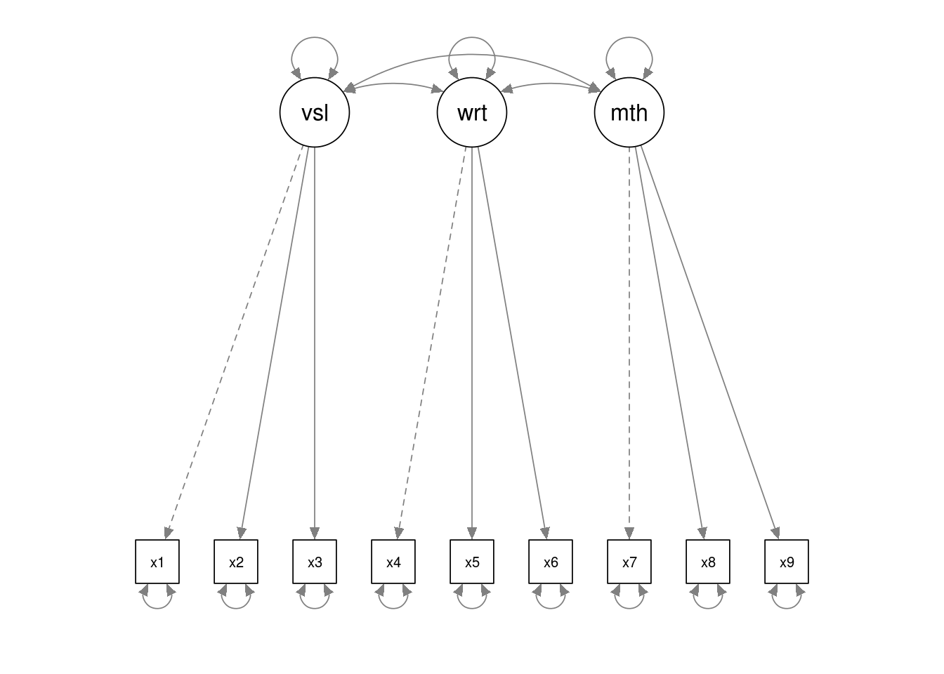
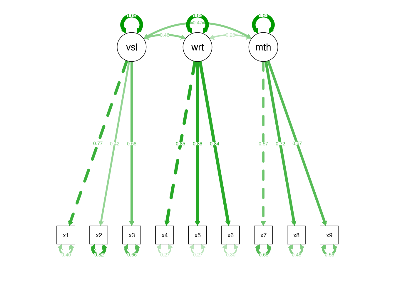
And for ‘final’ models we might want to overplot model parameter estimates (in this case, standardised):
# std refers to standardised estimates. "par" would plot
# the unstandardised estimates
semPlot::semPaths(hz.fit, "std")