Workflow
One big adjustment to make when moving away tools like SPSS is to find a ‘way of working’ that suits you.
We have often developed ways of working, saving, and communicating our work, and become comfortable with them. In part, these habits and routines may be attempts to work around limitations of these tools. But nevertheless, habits are easier to replace than break, so here’s an alternative model to adopt:
Work in RStudio, and use RMarkdown documents (see next sections).
Save your raw data in .csv format. Never edit data by hand unless absolutely necessary.
Use R to process your data and RMarkdown to document the process.
RMarkdown
Conventional statistics software like SPSS lacks a simple way to document and share your analyses, and make repeating or editing your work later very hard.
RMarkdown is a format for documenting and sharing statistical analyses.
This it might seem an odd place to start: we haven’t got anything to share yet! But using RMarkdown in RStudio provides a really nice way to work with data interactively and share our results, so we start as we mean to go on.
You are currently reading the output of an ‘RMarkdown’ document. An RMarkdown document mixes R code with Markdown:
- R is a computer language designed for working with data.
- Markdown is a simple text-based format which can include prose, hypertext links, images, and code (see http://commonmark.org/help/).
Like computer code, RMarkdown can be ‘run’ or ‘executed’. But in the language of RStudio, you ‘knit’ your RMarkdown to produce a finished document. This combines analyses, graphs, and explanatory text in a single pdf, html, or Word document which can be shared.
RStudio
RStudio is a special text editor that has been customised to make working with R easy. It can be installed on your own computer, or you can login to a shared RStudio server (for example, one run by your university) from a web browser. Either way the interface is largely the same and contains 4 main panels:
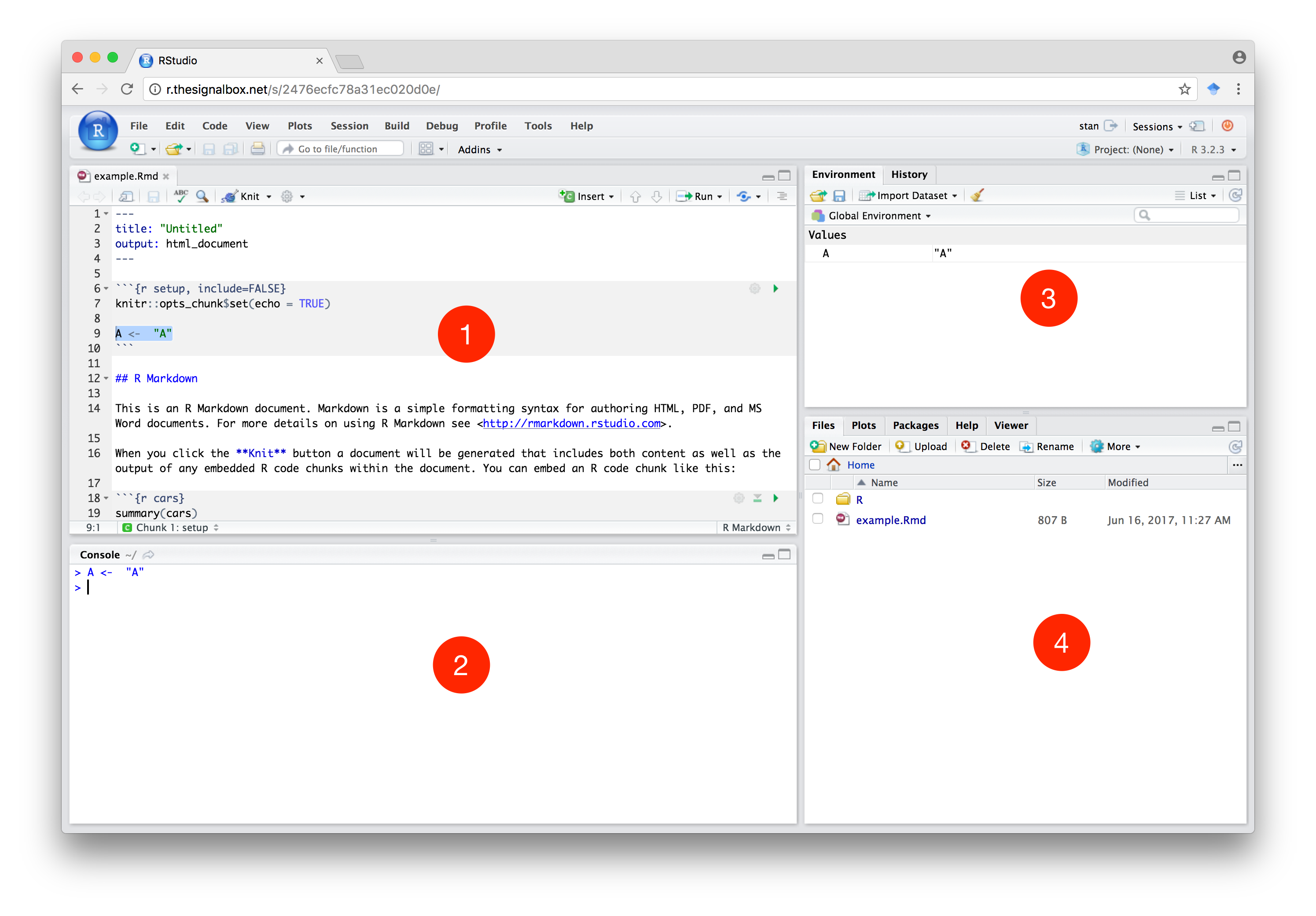
The figure above shows the main RStudio interface, comprising:
The main R-script or RMarkdown editor window. This is where you write commands, which can then be executed (to run the current line type ctrl-Enter or cmd-Enter on a Mac).
The R console, into which you can type R commands directly, and see the output of commands run in the script editor.
The ‘environment’ panel, which lists all the variables you have defined and currently available to use.
The files and help panel. Within this panel the ‘files’ tab enables you to open files stored on the server, in the current project, or elsewhere on your hard drive.
You can see a short video demonstrating the RStudio interface here:
The video:
- Shows you how to type commands into the Console and view the results.
- Run a plotting function, and see the result.
- Create RMarkdown file, and ‘Knit’ it to produce a document containing the results of your code and explanatory text.
Once you have watched the video:
- Open RStudio and create a new RMarkdown document.
- Edit some of the text, and press the
Knitbutton to see the results. - Edit some of the R blocks and see what happens.
Creating code chunks
To include R code within RMarkdown we write 3 backticks (```), followed by
{r}. We the include our R code, and close the block with 3 more backticks
(how to find the backtick on your keyboard).
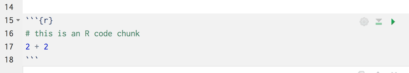
A code chunk in the RMarkdown editor
When a document including this chunk is run or ‘knitted’, the final result will
include the the line 2+2 followed by the number 4 on the next line. We can
use RMarkdown to ‘show our workings’: our analysis can be interleaved with
narrative text to explain or interpret the calculations.
More about RMarkdown
A more in depth explanation of RMarkdown is here: https://rmarkdown.rstudio.com, and a detailed user guide here: https://rmarkdown.rstudio.com/lesson-1.html