20 Confidence and Intervals
Some quick definitions to begin. Let’s say we have made an estimate from a model. To keep things simple, it could just be the sample mean.
A Confidence interval is the range within which we would expect the ‘true’ value to fall, 95% of the time, if we replicated the study.
A Prediction interval is the range within which we expect 95% of new observations to fall. If we’re considering the prediction interval for a specific point prediction (i.e. where we set predictors to specific values), then this interval woud be for new observations with the same predictor values.
A Bayesian Credible interval is the range of values within which we are 95% sure the true value lies, based on our prior knowledge and the data we have collected.
The problem with confidence intervals
Confidence intervals are helpful when we want to think about how precise our estimate is. For example, in an RCT we will want to estimate the difference between treatment groups, and it’s conceivable we would to want to know, for example, the range within which the true effect would fall 95% of the time if we replicated our study many times (although in reality, this isn’t a question many people would actually ask).
If we run a study with small N, intuitively we know that we have less information about the difference between our RCT treatments, and so we’d like the CI to expand accordingly.
So — all things being equal — the confidence interval reduces as we collect more data.
The problem with confidence intervals comes about because many researchers and clinicians read them incorrectly. Typically, they either:
Forget that the CI represents only the precision of the estimate. The CI doesn’t reflect how good our predictions for new observations will be.
Misinterpret the CI as the range in which we are 95% sure the true value lies.
Forgetting that the CI depends on sample size.
By forgetting that the CI contracts as the sample size increases, researchers can become overconfident about their ability to predict new observations. Imagine that we sample data from two populations with the same mean, but different variability:
set.seed(1234)
df <- expand.grid(v=c(1,3,3,3), i=1:1000) %>%
  as_data_frame %>%
  mutate(y = rnorm(length(.$i), 100, v)) %>%
  mutate(samp = factor(v, labels=c("Low variability", "High variability")))
Warning: `as_data_frame()` is deprecated, use `as_tibble()` (but mind the new semantics).
This warning is displayed once per session.
df %>%
ggplot(aes(y)) +
geom_histogram() +
facet_grid(~samp) +
scale_color_discrete("")
`stat_bin()` using `bins = 30`. Pick better value with `binwidth`.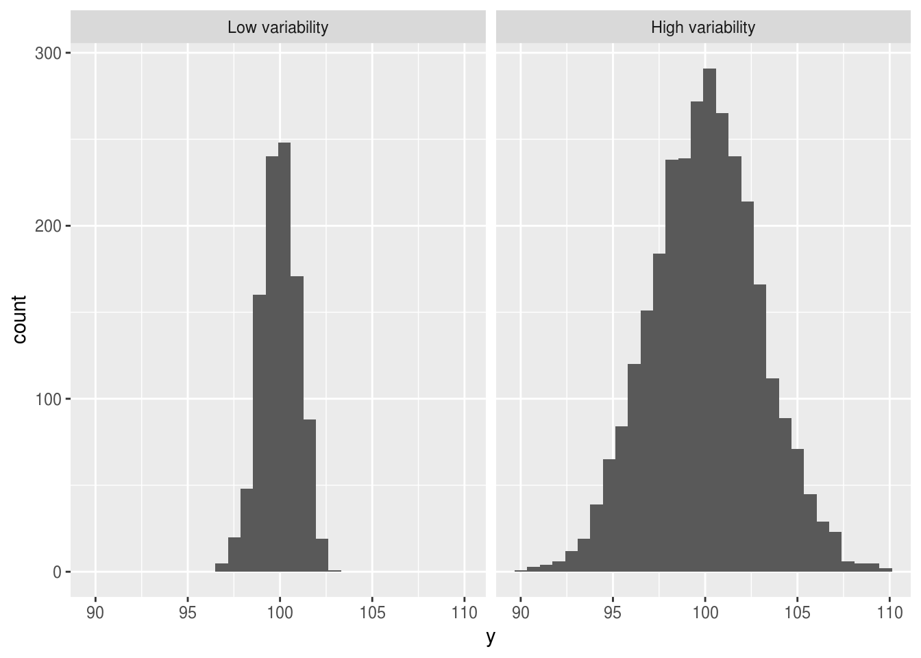
- If we sample 100 individuals from each population the confidence interval around the sample mean would be wider in the high variability group.
If we increase our sample size we would become more confident about the location of the mean, and this confidence interval would shrink.
But imagine taking a single new sample from either population. These samples would be new grey squares, which we place on the histograms above. It does not matter how much extra data we have collected in group B or how sure what the mean of the group is: We would always be less certain making predictions for new observations in the high variability group.
The important insight here is that if our data are noisy and highly variable we can never make firm predictions for new individuals, even if we collect so much data that we are very certain about the location of the mean.