t-tests

Visualising your data first

Before you run any tests it’s worth plotting your data.

Assuming you have a continuous outcome and categorical (binary) predictor (here we use a subset of the built in chickwts data), a boxplot can work well:

chicks.eating.beans <- chickwts %>%
  filter(feed %in% c("horsebean", "soybean"))

chicks.eating.beans %>%
  ggplot(aes(feed, weight)) +
  geom_boxplot()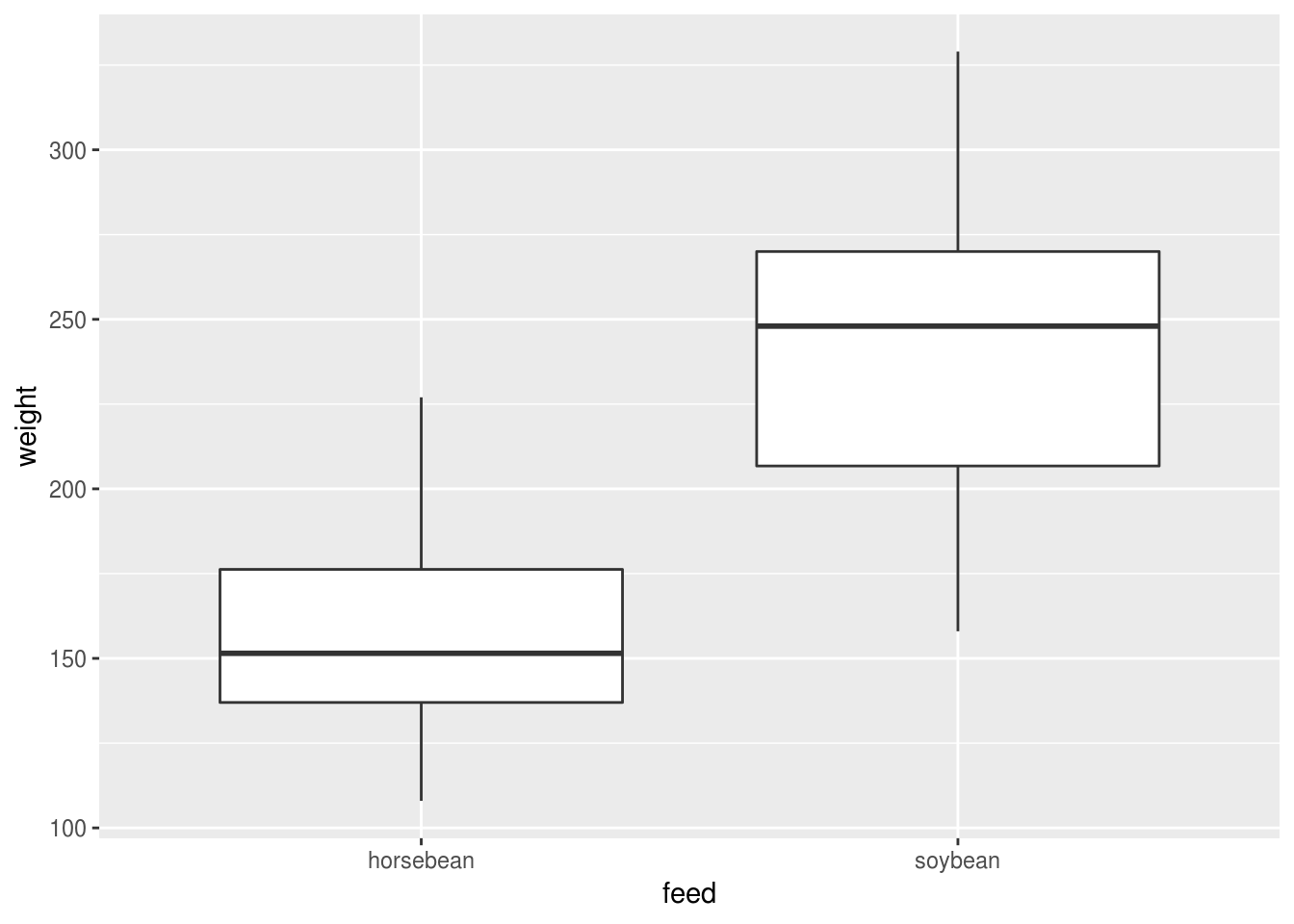

Figure 6.1: The box in a boxplot indictes the IQR; the whisker indicates the min/max values or 1.5 imes the IQR, whichever is the smaller. If there are outliers beyond 1.5 imes the IQR then they are shown as points.

Or a violin or bottle plot, which shows the distributions within each group and makes it relatively easy to check some of the main assumptions of the test:

chicks.eating.beans %>%
  ggplot(aes(feed, weight)) +
  geom_violin()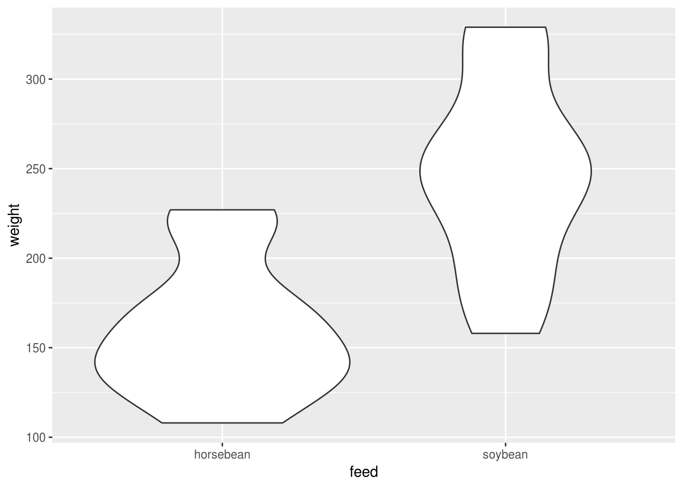

Layering boxes and bottles can work well too because it combines information about the distribution with key statistics like the median and IQR, and also because it scales reasonably well to multiple categories:

chickwts %>%
  ggplot(aes(feed, weight)) +
  geom_violin() +
  geom_boxplot(width=.1)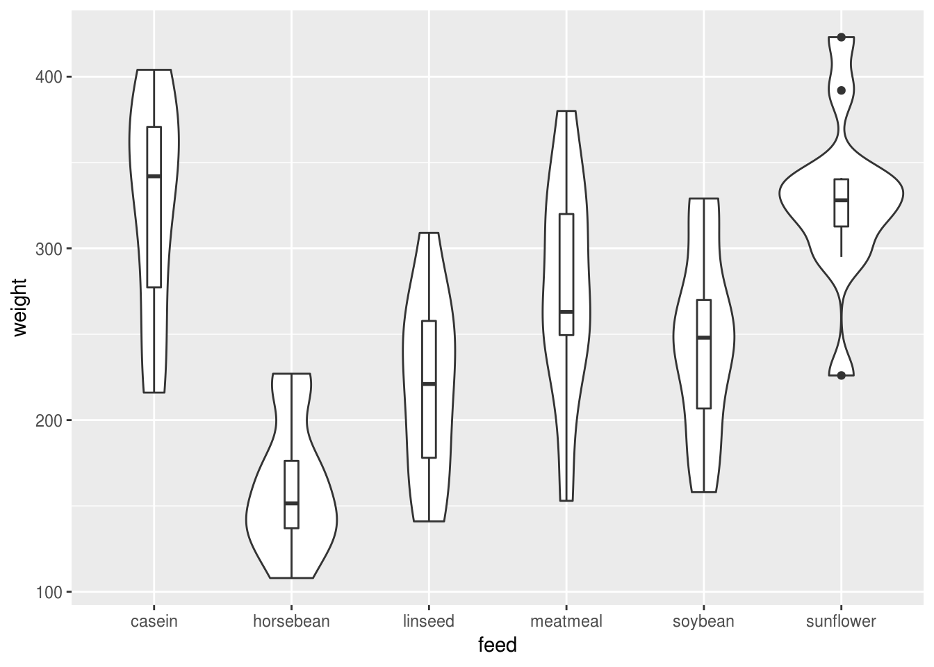

Running a t-test

Assuming you really do still want to run a null hypothesis test on one or two means, the t.test() function performs most common variants, illustrated below.

2 independent groups

Assuming your data are in long format:

t.test(weight ~ feed, data=chicks.eating.beans)

    Welch Two Sample t-test

data:  weight by feed
t = -4.5543, df = 21.995, p-value = 0.0001559
alternative hypothesis: true difference in means is not equal to 0
95 percent confidence interval:
 -125.49476  -46.96238
sample estimates:
mean in group horsebean   mean in group soybean 
               160.2000                246.4286 

Or equivalently, if your data are untidy and each group has it’s own column (e.g. chicks eating soybeans in one column and those eating horsebeans in another):

with(untidy.chicks, t.test(horsebean, soybean))

    Welch Two Sample t-test

data:  horsebean and soybean
t = -4.5543, df = 21.995, p-value = 0.0001559
alternative hypothesis: true difference in means is not equal to 0
95 percent confidence interval:
 -125.49476  -46.96238
sample estimates:
mean of x mean of y 
 160.2000  246.4286 

Equal or unequal variances?

By default R assumes your groups have unequal variances and applies an appropriate correction (you will notice the output labelled ‘Welch Two Sample t-test’).

You can turn this correction off (for example, if you’re trying to replcate an analysis done using the default settings in SPSS) but you probably do want to assume unequal variances [see @ruxton2006unequal].

Paired samples

If you have repeated measures on a sample you need a paired samples test.

# simulate paired samples in pre-post design
set.seed(1234)
baseline <- rnorm(50, 2.5, 1)
followup = baseline + rnorm(50, .5, 1)

# run paired samples test
t.test(baseline, followup, paired=TRUE)

    Paired t-test

data:  baseline and followup
t = -4.36, df = 49, p-value = 6.661e-05
alternative hypothesis: true difference in means is not equal to 0
95 percent confidence interval:
 -0.9342988 -0.3447602
sample estimates:
mean of the differences 
             -0.6395295 

Note that we could also ‘melt’ the data into long format and use the paired=TRUE argument with a formula:

long.form.data <- data_frame(baseline=baseline, follow=followup) %>%
  reshape2::melt()
Warning: `data_frame()` is deprecated, use `tibble()`.
This warning is displayed once per session.
No id variables; using all as measure variables

with(long.form.data, t.test(value~variable, paired=TRUE))

    Paired t-test

data:  value by variable
t = -4.36, df = 49, p-value = 6.661e-05
alternative hypothesis: true difference in means is not equal to 0
95 percent confidence interval:
 -0.9342988 -0.3447602
sample estimates:
mean of the differences 
             -0.6395295 

One-sample test

Sometimes you might want to compare a sample mean with a specific value:

# test if mean of `outcome` variable is different from 2
set.seed(1234)
test.scores <- rnorm(50, 2.5, 1)
t.test(test.scores, mu=2)

    One Sample t-test

data:  test.scores
t = 0.37508, df = 49, p-value = 0.7092
alternative hypothesis: true mean is not equal to 2
95 percent confidence interval:
 1.795420 2.298474
sample estimates:
mean of x 
 2.046947 

---

title: ‘Regression in R’

---