Anova ‘Cookbook’

This section is intended as a shortcut to running Anova for a variety of common types of model. If you want to understand more about what you are doing, read the section on principles of Anova in R first, or consult an introductory text on Anova which covers Anova [e.g. @howell2012statistical].

Between-subjects Anova

Oneway Anova (> 2 groups)

If your design has more than 2 groups then you should use oneway Anova.

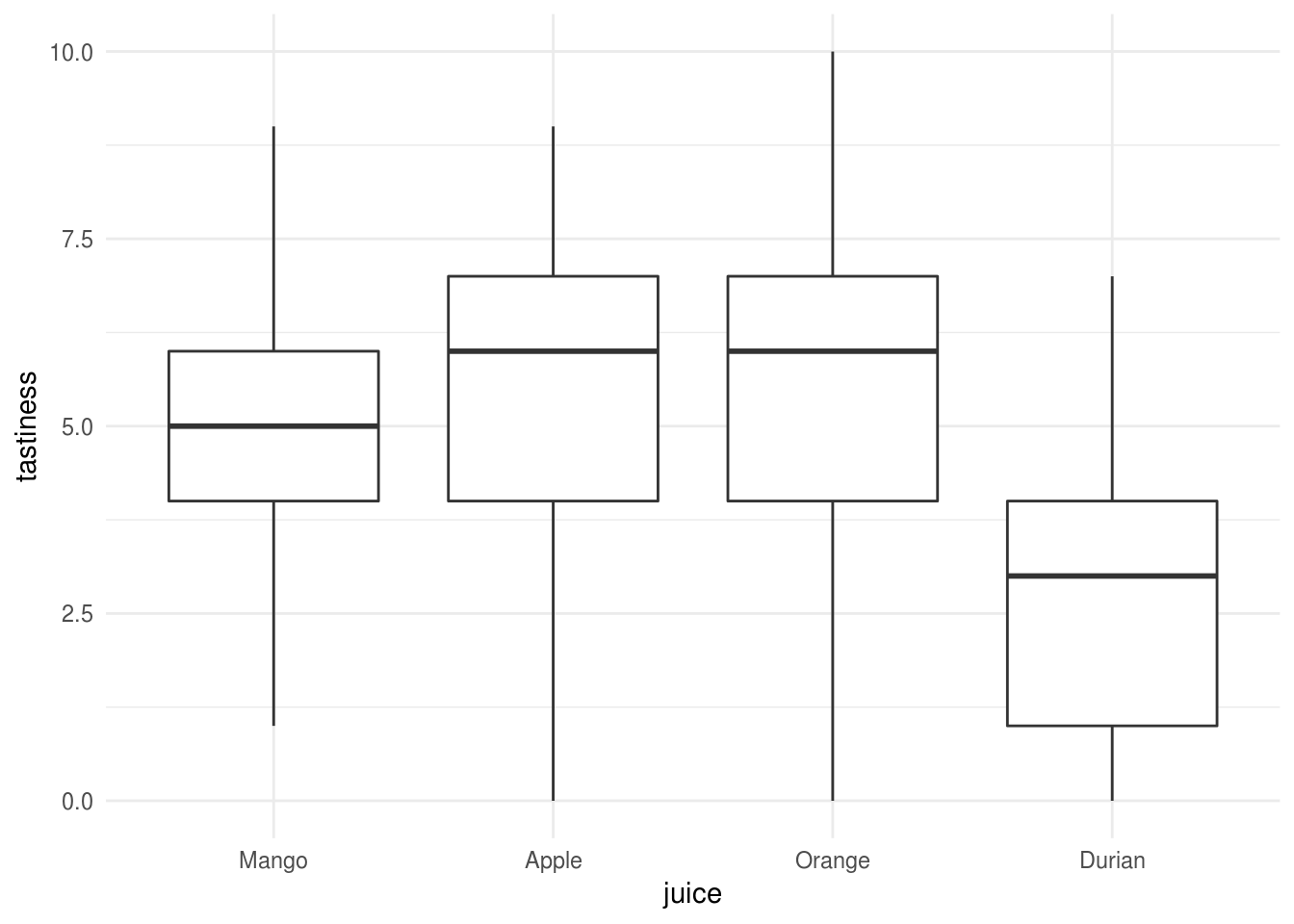
Let’s say we asked people to taste 1 of 4 fruit juices, and rate how tasty it was on a scale from 0 to 10:

We can run a oneway Anova with type 3 sums of squares using the Anova function from the car:: package:

juice.lm <- lm(tastiness ~ juice, data=tasty.juice)
juice.anova <- car::Anova(juice.lm, type=3)
juice.anova
Anova Table (Type III tests)

Response: tastiness
            Sum Sq Df  F value    Pr(>F)    
(Intercept) 615.04  1 114.4793 < 2.2e-16 ***
juice       128.83  3   7.9932 8.231e-05 ***
Residuals   515.76 96                       
---
Signif. codes:  0 '***' 0.001 '**' 0.01 '*' 0.05 '.' 0.1 ' ' 1

And we could compute the contasts for each fruit against the others (the grand mean):

juice.lsm <- emmeans::emmeans(juice.lm, pairwise~juice, adjust="fdr")
juice.contrasts <- emmeans::contrast(juice.lsm, "eff")
juice.contrasts$contrasts
 contrast               estimate    SE df t.ratio p.value
 Mango - Apple effect      -1.90 0.637 96 -2.982  0.0060 
 Mango - Orange effect     -1.54 0.512 96 -3.005  0.0060 
 Mango - Durian effect      1.02 0.346 96  2.952  0.0060 
 Apple - Orange effect     -0.78 0.637 96 -1.224  0.2239 
 Apple - Durian effect      1.78 0.512 96  3.473  0.0046 
 Orange - Durian effect     1.42 0.637 96  2.229  0.0338 

P value adjustment: fdr method for 6 tests 

We found a significant main effect of juice, r apastats::describe.Anova(juice.anova, 2). Followup tests (adjusted for false discovery rate) indicated that only Durian differed from the other juices, and was rated a significantly less tasty Mango, Apple, and Orange juice.

Factorial Anova

We are using a dataset from Howell [@howell2012statistical, chapter 13]: an experiment which recorded Recall among young v.s. older adults (Age) for each of 5 conditions.

These data would commonly be plotted something like this:

eysenck <- readRDS("data/eysenck.Rdata")
eysenck %>%
  ggplot(aes(Condition, Recall, group=Age, color=Age)) +
  stat_summary(geom="pointrange", fun.data = mean_cl_boot) +
  ylab("Recall (95% CI)") +
  xlab("")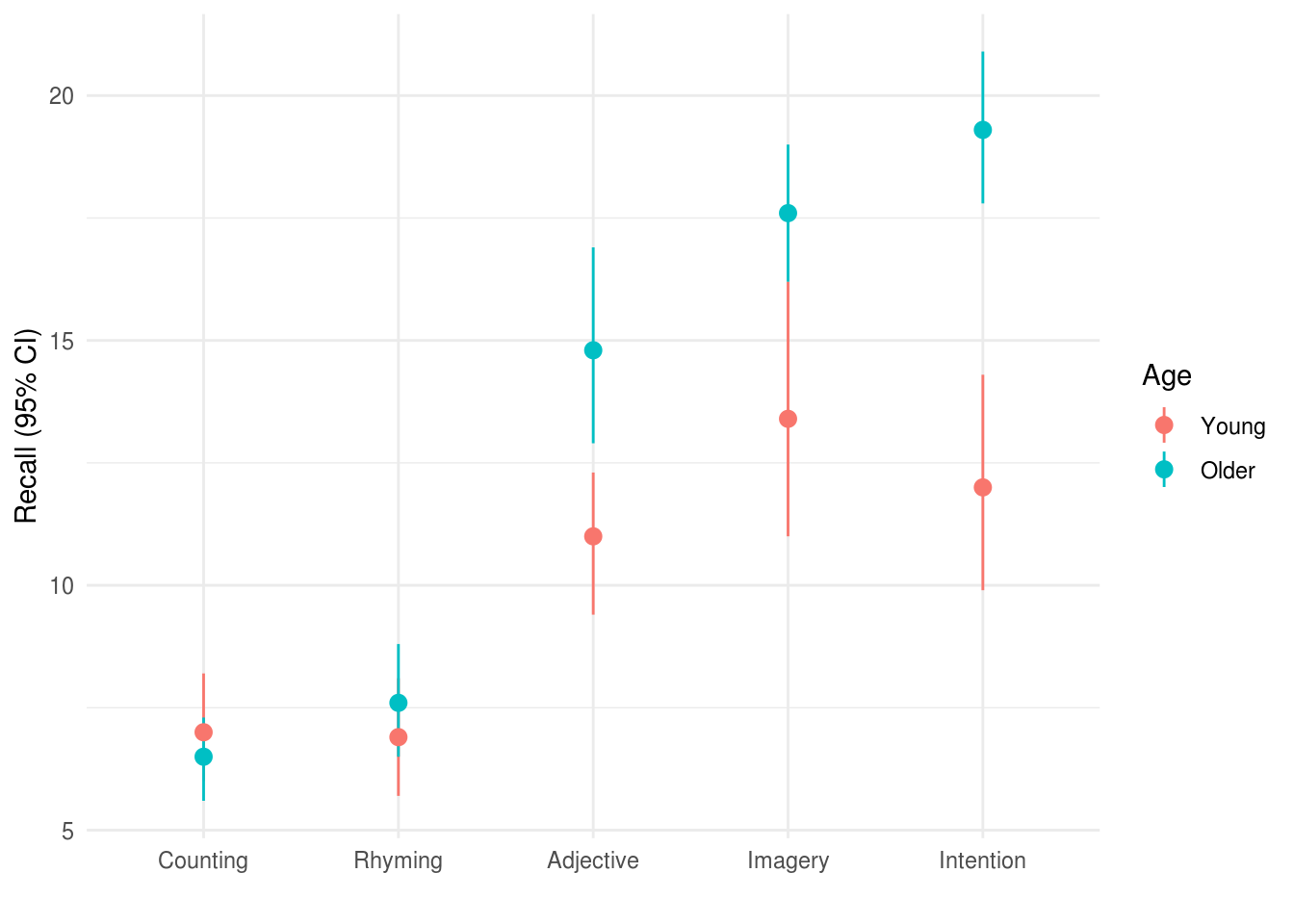

Visual inspection of the data (see Figure X) suggested that older adults recalled more words than younger adults, and that this difference was greatest for the intention, imagery, and adjective conditions. Recall peformance was worst in the counting and rhyming conditions.

Or alternatively if we wanted to provde a better summary of the distribution of the raw data we could use a boxplot:

eysenck %>%
  ggplot(aes(Age, Recall)) +
  geom_boxplot(width=.33) +
  facet_grid(~Condition) +
  ylab("Recall (95% CI)") +
  xlab("")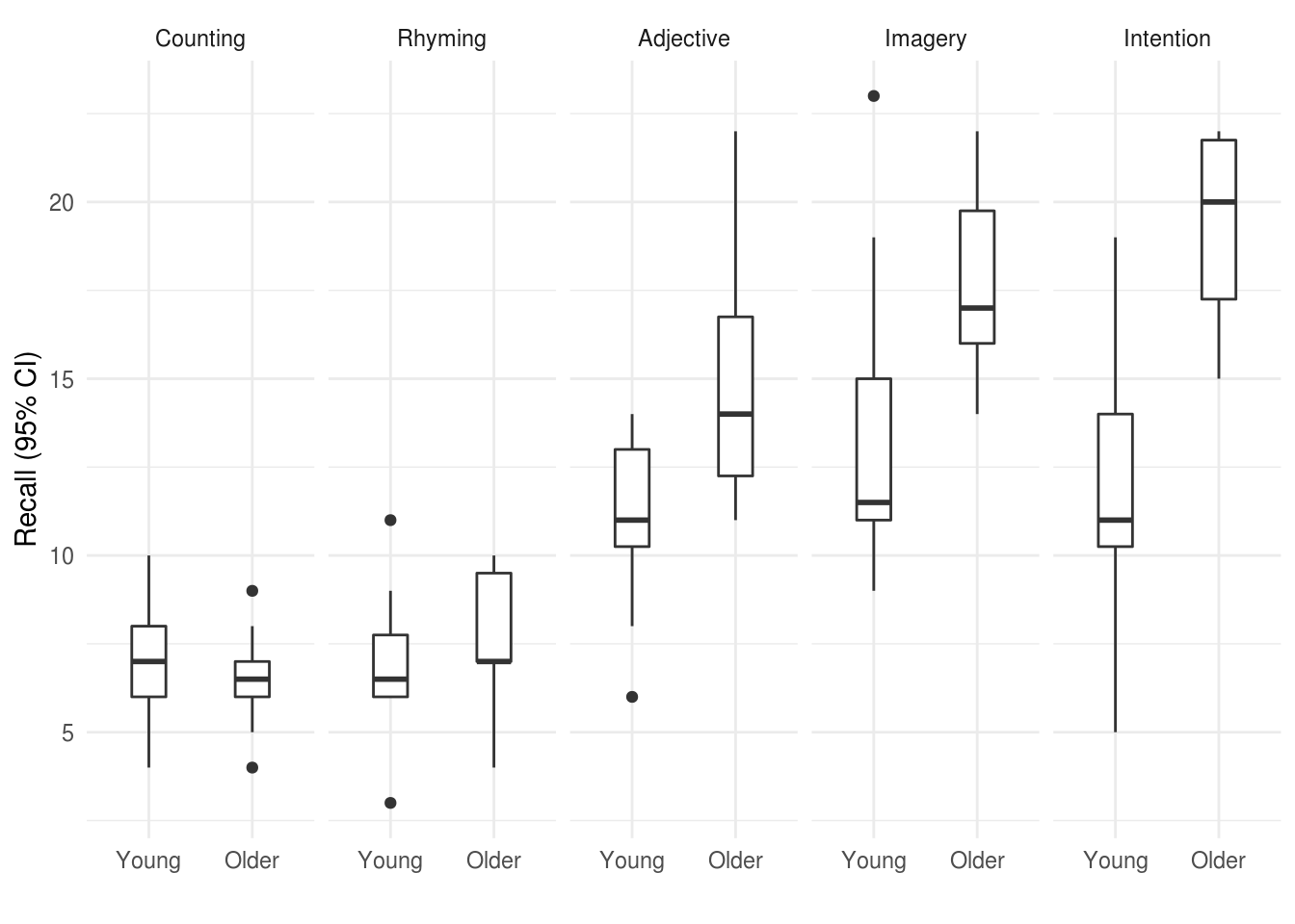

Figure 2.2: Boxplot for recall in older and young adults, by condition.

We can run a linear model including the effect of Age and Condition and the interaction of these variables, and calculate the Anova:

eysenck.model <- lm(Recall~Age*Condition, data=eysenck)
car::Anova(eysenck.model, type=3)
Anova Table (Type III tests)

Response: Recall
              Sum Sq Df F value    Pr(>F)    
(Intercept)   490.00  1 61.0550  9.85e-12 ***
Age             1.25  1  0.1558 0.6940313    
Condition     351.52  4 10.9500  2.80e-07 ***
Age:Condition 190.30  4  5.9279 0.0002793 ***
Residuals     722.30 90                      
---
Signif. codes:  0 '***' 0.001 '**' 0.01 '*' 0.05 '.' 0.1 ' ' 1

Repeated measures or ‘split plot’ designs

It might be controversial to say so, but the tools to run traditional repeat measures Anova in R are a bit of a pain to use. Although there are numerous packages simplify the process a little, their syntax can be obtuse or confusing. To make matters worse, various textbooks, online guides and the R help files themselves show many ways to achieve the same ends, and it can be difficult to follow the differences between the underlying models that are run.

At this point, given the many other advantages of linear mixed models over traditional repeated measures Anova, and given that many researchers abuse traditional Anova in practice (e.g. using it for unbalanced data, or where some data are missing), the recommendation here is to simply give up and learn how to run linear mixed models. These can (very closely) replicate traditional Anova approaches, but also:

• Handle missing data or unbalanced designs gracefully and efficiently.

• Be expanded to include multiple levels of nesting. For example, allowing pupils to be nested within classes, within schools. Alternatively multiple measurements of individual patients might be clustered by hospital or therapist.

• Allow time to be treated as a continuous variable. For example, time can be modelled as a slope or some kind of curve, rather than a fixed set of observation-points. This can be more parsimonious, and more flexible when dealing with real-world data (e.g. from clinical trials).

It would be best at this point to jump straight to the main section multilevel or mixed-effects models, but to give one brief example of mixed models in use:

The sleepstudy dataset in the lme4 package provides reaction time data recorded from participants over a period of 10 days, during which time they were deprived of sleep.

lme4::sleepstudy %>%
  head(12) %>%
  pander

Reaction	Days	Subject
249.6	0	308
258.7	1	308
250.8	2	308
321.4	3	308
356.9	4	308
414.7	5	308
382.2	6	308
290.1	7	308
430.6	8	308
466.4	9	308
222.7	0	309
205.3	1	309

We can plot these data to show the increase in RT as sleep deprivation continues:

lme4::sleepstudy %>%
  ggplot(aes(factor(Days), Reaction)) +
  geom_boxplot() +
  xlab("Days") + ylab("RT (ms)") +
  geom_label(aes(y=400, x=2, label="you start to\nfeel bad here"), color="red") +
  geom_label(aes(y=450, x=9, label="imagine how bad\nyou feel by this point"), color="red")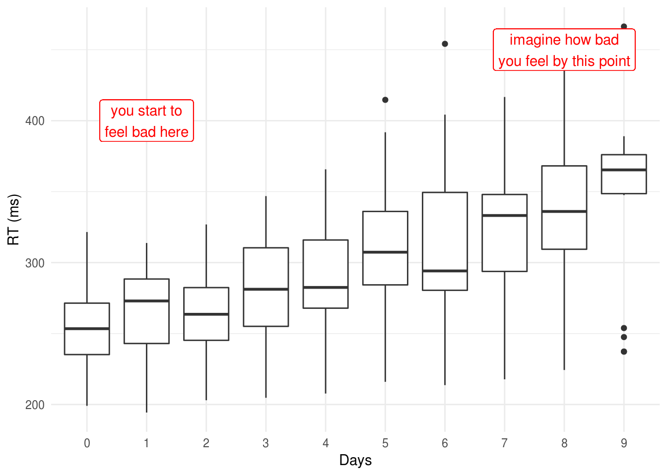

If we want to test whether there are significant differences in RTs between Days, we could fit something very similar to a traditional repeat measures Anova using the lme4::lmer() function, and obtain an Anova table for the model using the special anova() function which is added by the lmerTest package:

sleep.model <- lmer(Reaction ~ factor(Days) + (1 | Subject), data=lme4::sleepstudy)
anova(sleep.model)
Type III Analysis of Variance Table with Satterthwaite's method
             Sum Sq Mean Sq NumDF DenDF F value    Pr(>F)    
factor(Days) 166235   18471     9   153  18.703 < 2.2e-16 ***
---
Signif. codes:  0 '***' 0.001 '**' 0.01 '*' 0.05 '.' 0.1 ' ' 1

Traditional repeated measures Anova

If you really need to fit the traditional repeated measures Anova (e.g. your supervisor/reviewer has asked you to) then you should use either the afex:: or ez:: packages.

Let’s say we have an experiment where we record reaction 25 times (Trial) before and after (Time = {1, 2}) one of 4 experimental manipulations (Condition = {1,2,3,4}). You have 12 participants in each condition and no missing data:

expt.data %>%
  ggplot(aes(Condition, RT)) +
  geom_boxplot() +
  facet_wrap(~paste("Time", time))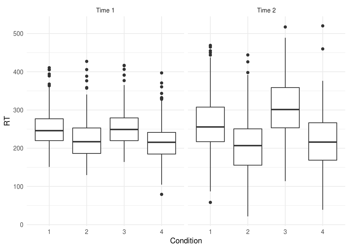

We want to use our repeated measurements before and after the experimental interventions to increase the precision of our estimate of the between-condition differences.

Our first step is to aggregate RTs for the multiple trials, taking the mean across all trials at a particular time:

expt.data.agg <- expt.data %>%
  group_by(Condition, person, time) %>%
  summarise(RT=mean(RT))

head(expt.data.agg)
# A tibble: 6 x 4
# Groups:   Condition, person [3]
  Condition person time     RT
  <fct>     <fct>  <fct> <dbl>
1 1         1      1      270.
2 1         1      2      246.
3 1         2      1      257.
4 1         2      2      247.
5 1         3      1      239.
6 1         3      2      249.

Because our data are still in long form (we have two rows per person), we have to explicitly tell R that time is a within subject factor. Using the afex:: package we would write:

expt.afex <- afex::aov_car(RT ~ Condition * time + Error(person/time),
                           data=expt.data.agg)
expt.afex$anova_table %>%
  pander(caption="`afex::aov_car` output.")

afex::aov_car output.

	num Df	den Df	MSE	F	ges	Pr(>F)
Condition	3	44	160.6	142.1	0.8289	1.193e-22
time	1	44	160.5	20.85	0.1915	3.987e-05
Condition:time	3	44	160.5	29.42	0.5006	1.358e-10

Using the ez:: package we would write:

expt.ez <- ez::ezANOVA(data=expt.data.agg,
            dv = RT,
            wid = person,
            within = time,
            between = Condition)

expt.ez$ANOVA %>%
  pander(caption="`ez::ezANOVA` output.")

ez::ezANOVA output.

	Effect	DFn	DFd	F	p	p<.05	ges
2	Condition	3	44	142.1	1.193e-22	*	0.8289
3	time	1	44	20.85	3.987e-05	*	0.1915
4	Condition:time	3	44	29.42	1.358e-10	*	0.5006

These are the same models: any differences in the output are simply due to rounding. You should use whichever of ez:: and afex:: you find easiest to understand

The ges column is the generalised eta squared effect-size measure, which is preferable to the partial eta-squared reported by SPSS [@bakeman2005recommended].

But what about [insert favourite R package for Anova]?

Lots of people like ez::ezANOVA and other similar packages. My problem with ezANOVA is that it doesn’t use formulae to define the model and for this reason encourages students to think of Anova as something magical and separate from linear models and regression in general.

This guide is called ‘just enough R’, so I’ve mostly chosen to show only car::Anova because I find this the most coherent method to explain. Using formulae to specify the model reinforces a technique which is useful in many other contexts. I’ve make an exception for repeated because many people find specifying the error structure explicitly confusing and hard to get right, and so ez:: may be the best option in these cases.

Comparison with a multilevel model

For reference, a broadly equivalent (although not identical) multilevel model would be:

expt.mlm  <- lmer(RT ~ Condition * time + (1|person),
    data=expt.data.agg)

anova(expt.mlm) %>%
    pander()

Type III Analysis of Variance Table with Satterthwaite’s method

	Sum Sq	Mean Sq	NumDF	DenDF	F value	Pr(>F)
Condition	68424	22808	3	41.22	142.1	9.189e-22
time	3346	3346	1	41.21	20.84	4.443e-05
Condition:time	14167	4722	3	41.21	29.41	2.486e-10

Although with a linear mixed model it would also be posible to analyse the trial-by-trial data. Let’s hypothesise, for example, that subjects in Conditions 2 and 4 experienced a ‘practice effect’, such that their RTs reduced over multiple trials. If we plot the data, we can see this suspicion may be supported (how conveninent!):

ggplot(expt.data,
  aes(trial, RT)) +
  geom_smooth() +
  facet_wrap(~paste("Condition", Condition))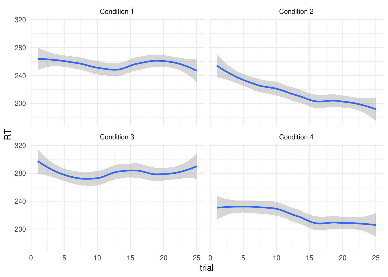

If we wanted to replicate the aggregated RM Anova models shown above we could write:

options(contrasts = c("contr.sum", "contr.poly"))
expt.mlm2 <- lmer(RT ~ Condition * time + (time|person), data=expt.data)
anova(expt.mlm2)
Type III Analysis of Variance Table with Satterthwaite's method
                Sum Sq Mean Sq NumDF  DenDF F value    Pr(>F)    
Condition      1331102  443701     3 67.844 118.473 < 2.2e-16 ***
time             65082   65082     1 67.921  17.378 8.875e-05 ***
Condition:time  275524   91841     3 67.921  24.523 7.285e-11 ***
---
Signif. codes:  0 '***' 0.001 '**' 0.01 '*' 0.05 '.' 0.1 ' ' 1

But we can now add a continuous predictor for trial:

expt.mlm.bytrial <- lmer(RT ~ Condition * time * trial +
    (time|person),
    data=expt.data)

anova(expt.mlm.bytrial)
Type III Analysis of Variance Table with Satterthwaite's method
                     Sum Sq Mean Sq NumDF   DenDF F value    Pr(>F)    
Condition            150397   50132     3  658.88 13.6651 1.174e-08 ***
time                  21561   21561     1  659.67  5.8772   0.01561 *  
trial                112076  112076     1 2340.00 30.5499 3.615e-08 ***
Condition:time        81051   27017     3  659.67  7.3643 7.362e-05 ***
Condition:trial       90818   30273     3 2340.00  8.2517 1.845e-05 ***
time:trial              178     178     1 2340.00  0.0485   0.82576    
Condition:time:trial   5940    1980     3 2340.00  0.5397   0.65509    
---
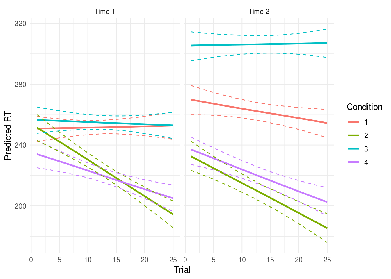
Signif. codes:  0 '***' 0.001 '**' 0.01 '*' 0.05 '.' 0.1 ' ' 1

The significant Condition:trial term indicates that there was a difference in the practice effects between the experimental conditions.

We found a significant interaction between condition and the linear term for trial number, F(3, 2340.18) = 10.83, p < .001. We explored this effect by plotting model-estimated reaction times for each group for trials 1 through 25 (see Figure X): participants in condition 2 and 4 exprienced a greater reduction in RTs across trial, suggesting a larger practice effect for these conditions.

See the multilevel models section for more details, including analyses which allow the effects of interventions to vary between participants (i.e., relaxing the assumption that an intervention will be equally effective for all participants).

RM Anova v.s. multilevel models

• The RM Anova is perhaps more familiar, and may be conventional in your field which can make peer review easier (although in other fields mixed models are now expected where the design warrants it).

• RM Anova requires complete data: any participant with any missing data will be dropped from the analysis. This is problematic where data are expensive to collect, and where data re unlikely to be missing at random, for example in a clinical trial. In these cases RM Anova may be less efficient and more biased than an equivalent multilevel model.

• There is no simple way of calculating effect size measures like eta² from the lmer model. This may or may not be a bad thing. @baguley2009standardized, for example, recommends reporting simple (rather than standardised) effect size measures, and is easily done by making predictions from the model.