Path models
Path models are an extension of linear regression, but where multiple observed variables can be considered as ‘outcomes’.
Because the terminology of outcomes v.s. predictors breaks down when variables can be both outcomes and predictors at the same time, it’s normal to distinguish instead between:
Exogenous variables: those which are not predicted by any other
Endogenous variables: variables which do have predictors, and may or may not predict other variales
Defining a model
To define a path model, lavaan requires that you specify the relationships
between variables in a text format. A full
guide to this lavaan model syntax
is available on the project website.
For path models the format is very simple, and resembles a series of linear models, written over several lines, but in text rather than as a model formula:
# define the model over multiple lines for clarity
mediation.model <- "
  y ~ x + m
  m ~ x
"
In this case the ~ symbols just means ‘regressed on’ or ‘is predicted by’. The
model in the example above defines that our outcome y is predicted by both x
and m, and that x also predicts m. You might recognise this as a
mediation model.
Make sure you include the closing quote symbol, and also be careful when running the code which defines the model. RStdudio can sometimes get confused and only run some of the lines, leading to errors. The simplest solution is to select the entire block explicitly and run that.
To fit the model we pass the model specification and the data to the sem()
function:
mediation.fit <- sem(mediation.model, data=mediation.df)As we did for linear regression models, we have saved
the model fit object into a variable, here named mediation.fit.
To display the model results we can use summary(). The key section of the
output to check is the table listed ‘Regressions’, which lists the regression
parameters for the predictors for each of the endogenous variables.
summary(mediation.fit)
lavaan 0.6-3 ended normally after 12 iterations

  Optimization method                           NLMINB
  Number of free parameters                          5

  Number of observations                           200

  Estimator                                         ML
  Model Fit Test Statistic                       0.000
  Degrees of freedom                                 0
  Minimum Function Value               0.0000000000000

Parameter Estimates:

  Information                                 Expected
  Information saturated (h1) model          Structured
  Standard Errors                             Standard

Regressions:
                   Estimate  Std.Err  z-value  P(>|z|)
  y ~
    x                 0.166    0.075    2.198    0.028
    m                 0.190    0.070    2.721    0.007
  m ~
    x                 0.530    0.067    7.958    0.000

Variances:
                   Estimate  Std.Err  z-value  P(>|z|)
   .y                 0.967    0.097   10.000    0.000
   .m                 0.993    0.099   10.000    0.000
From this table we can see that both x and m are significant predictors of
y, and that x also predicts m. This implie that mediation is taking place,
but see the mediation chapter for details of testing indirect
effects in lavaan.
Where’s the intercept?
Path analysis is part of the set of techniques often termed ‘covariance modelling’. As the name implies the primary focus here is the relationships between variables, and less so the mean-structure of the variables. In fact, by default the software first creates the covariance matrix of all the variables in the model, and the fit is based only on these values, plus the sample sizes (in early SEM software you typically had to provide the covariance matrix directly, rather than working with the raw data).
Nonetheless, because path analysis is an extension of regression techniques it
is possible to request that intercepts are included in the model, and means
estimated, by adding meanstructure=TRUE to the sem() function
(see the lavaan manual for details).
In the output below we now also see a table labelled ‘Intercepts’ which gives the mean values of each variable when it’s predictors are zero (just like in linear regression):
mediation.fit.means <- sem(mediation.model,
                           meanstructure=T,
                           data=mediation.df)

summary(mediation.fit.means)
lavaan 0.6-3 ended normally after 16 iterations

  Optimization method                           NLMINB
  Number of free parameters                          7

  Number of observations                           200

  Estimator                                         ML
  Model Fit Test Statistic                       0.000
  Degrees of freedom                                 0
  Minimum Function Value               0.0000000000000

Parameter Estimates:

  Information                                 Expected
  Information saturated (h1) model          Structured
  Standard Errors                             Standard

Regressions:
                   Estimate  Std.Err  z-value  P(>|z|)
  y ~
    x                 0.166    0.075    2.198    0.028
    m                 0.190    0.070    2.721    0.007
  m ~
    x                 0.530    0.067    7.958    0.000

Intercepts:
                   Estimate  Std.Err  z-value  P(>|z|)
   .y                10.629    0.362   29.323    0.000
   .m                 5.097    0.070   72.298    0.000

Variances:
                   Estimate  Std.Err  z-value  P(>|z|)
   .y                 0.967    0.097   10.000    0.000
   .m                 0.993    0.099   10.000    0.000
Tables of model coefficients
If you want to present results from these models in table format, the
parameterEstimates() function is useful to extract the relevant numbers as a
dataframe. We can then manipulate and present this table as we would any other
dataframe.
In the example below we extract the parameter estimates, select only the
regression parameters (~) and remove some of the columns to make the final
output easier to read:
parameterEstimates(mediation.fit.means) %>%
  as_tibble() %>%
  filter(op=="~") %>%
  mutate(Term=paste(lhs, op, rhs)) %>%
  rename(estimate=est,
         p=pvalue) %>%
  select(Term, estimate, z, p) %>%
pander::pander(caption="Regression parameters from `mediation.fit`")| Term | estimate | z | p |
|---|---|---|---|
| y ~ x | 0.1657 | 2.198 | 0.02797 |
| y ~ m | 0.1899 | 2.721 | 0.006515 |
| m ~ x | 0.5298 | 7.958 | 1.776e-15 |
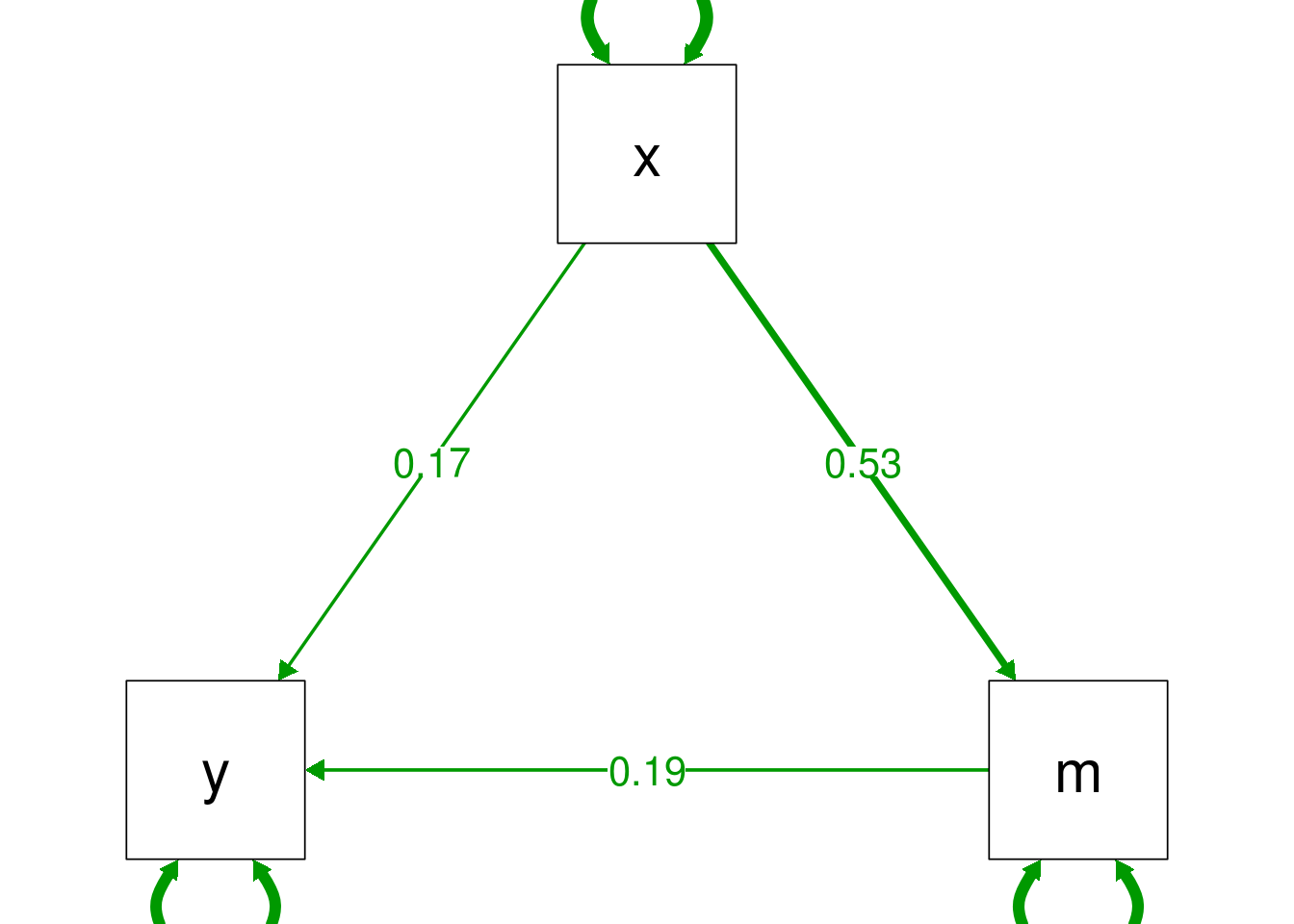
Diagrams
Because describing path, CFA and SEM models in words can be tedious and difficult for readers to follow it is conventional to include a diagram of (at least) your final model, and perhaps also initial or alternative models.
The semPlot:: package makes this relatively easy: passing a fitted lavaan
model to the semPaths() function produces a line drawing, and gives the option
to overlap raw or standardised coefficients over this drawing:
# unfortunately semPaths plots very small by default, so we set
# some extra parameters to increase the size to make it readable
semPlot::semPaths(mediation.fit, "par",
             sizeMan = 15, sizeInt = 15, sizeLat = 15,
             edge.label.cex=1.5,
             fade=FALSE)