Missing values
Missing values aren’t a data type as such, but are an important concept in R; the way different functions handle missing values can be both helpful and frustrating in equal measure.
Missing values in a vector are denoted by the letters NA, but notice that these letters are unquoted. That is to say NA is not the same as "NA"!
To check for missing values in a vector (or dataframe column) we use the is.na() function:
nums.with.missing <- c(1, 2, NA)
nums.with.missing
[1]  1  2 NA

is.na(nums.with.missing)
[1] FALSE FALSE  TRUE
Here the is.na() function has tested whether each item in our vector called nums.with.missing is missing. It returns a new vector with the results of each test: either TRUE or FALSE.
We can also use the negation operator, the ! symbol to reverse the meaning of is.na. So we can read !is.na(nums) as “test whether the values in nums are NOT missing”:
# test if missing
is.na(nums.with.missing)
[1] FALSE FALSE  TRUE

# test if NOT missing (note the exclamation mark in front of the function)
!is.na(nums.with.missing)
[1]  TRUE  TRUE FALSE
We can use the is.na() function as part of dplyr filters:
airquality %>%
  filter(is.na(Solar.R)) %>%
  head(3) %>%
pander| Ozone | Solar.R | Wind | Temp | Month | Day |
|---|---|---|---|---|---|
| NA | NA | 14.3 | 56 | 5 | 5 |
| 28 | NA | 14.9 | 66 | 5 | 6 |
| 7 | NA | 6.9 | 74 | 5 | 11 |
Or to select only cases without missing values for a particular variable:
airquality %>%
  filter(!is.na(Solar.R)) %>%
  head(3) %>%
pander| Ozone | Solar.R | Wind | Temp | Month | Day |
|---|---|---|---|---|---|
| 41 | 190 | 7.4 | 67 | 5 | 1 |
| 36 | 118 | 8 | 72 | 5 | 2 |
| 12 | 149 | 12.6 | 74 | 5 | 3 |
Complete cases
Sometimes we want to select only rows which have no missing values — i.e. complete cases.
The complete.cases function accepts a dataframe (or matrix) and tests whether each row is complete. It returns a vector with a TRUE/FALSE result for each row:
complete.cases(airquality) %>%
  head
[1]  TRUE  TRUE  TRUE  TRUE FALSE FALSE
This can also be useful in dplyr filters. Here we show all the rows which are not complete (note the exclamation mark):
airquality %>%
  filter(!complete.cases(airquality))
   Ozone Solar.R Wind Temp Month Day
1     NA      NA 14.3   56     5   5
2     28      NA 14.9   66     5   6
3     NA     194  8.6   69     5  10
4      7      NA  6.9   74     5  11
5     NA      66 16.6   57     5  25
6     NA     266 14.9   58     5  26
7     NA      NA  8.0   57     5  27
8     NA     286  8.6   78     6   1
9     NA     287  9.7   74     6   2
10    NA     242 16.1   67     6   3
11    NA     186  9.2   84     6   4
12    NA     220  8.6   85     6   5
13    NA     264 14.3   79     6   6
14    NA     273  6.9   87     6   8
15    NA     259 10.9   93     6  11
16    NA     250  9.2   92     6  12
17    NA     332 13.8   80     6  14
18    NA     322 11.5   79     6  15
19    NA     150  6.3   77     6  21
20    NA      59  1.7   76     6  22
21    NA      91  4.6   76     6  23
22    NA     250  6.3   76     6  24
23    NA     135  8.0   75     6  25
24    NA     127  8.0   78     6  26
25    NA      47 10.3   73     6  27
26    NA      98 11.5   80     6  28
27    NA      31 14.9   77     6  29
28    NA     138  8.0   83     6  30
29    NA     101 10.9   84     7   4
30    NA     139  8.6   82     7  11
31    NA     291 14.9   91     7  14
32    NA     258  9.7   81     7  22
33    NA     295 11.5   82     7  23
34    78      NA  6.9   86     8   4
35    35      NA  7.4   85     8   5
36    66      NA  4.6   87     8   6
37    NA     222  8.6   92     8  10
38    NA     137 11.5   86     8  11
39    NA      64 11.5   79     8  15
40    NA     255 12.6   75     8  23
41    NA     153  5.7   88     8  27
42    NA     145 13.2   77     9  27
Sometimes it’s convenient to use the . (period) to represent the output from the previous pipe command. For example, we could rewrite the previous example as:
airquality %>%
  filter(!complete.cases(.))  # note the . (period) here in place of `airmiles`
   Ozone Solar.R Wind Temp Month Day
1     NA      NA 14.3   56     5   5
2     28      NA 14.9   66     5   6
3     NA     194  8.6   69     5  10
4      7      NA  6.9   74     5  11
5     NA      66 16.6   57     5  25
6     NA     266 14.9   58     5  26
7     NA      NA  8.0   57     5  27
8     NA     286  8.6   78     6   1
9     NA     287  9.7   74     6   2
10    NA     242 16.1   67     6   3
11    NA     186  9.2   84     6   4
12    NA     220  8.6   85     6   5
13    NA     264 14.3   79     6   6
14    NA     273  6.9   87     6   8
15    NA     259 10.9   93     6  11
16    NA     250  9.2   92     6  12
17    NA     332 13.8   80     6  14
18    NA     322 11.5   79     6  15
19    NA     150  6.3   77     6  21
20    NA      59  1.7   76     6  22
21    NA      91  4.6   76     6  23
22    NA     250  6.3   76     6  24
23    NA     135  8.0   75     6  25
24    NA     127  8.0   78     6  26
25    NA      47 10.3   73     6  27
26    NA      98 11.5   80     6  28
27    NA      31 14.9   77     6  29
28    NA     138  8.0   83     6  30
29    NA     101 10.9   84     7   4
30    NA     139  8.6   82     7  11
31    NA     291 14.9   91     7  14
32    NA     258  9.7   81     7  22
33    NA     295 11.5   82     7  23
34    78      NA  6.9   86     8   4
35    35      NA  7.4   85     8   5
36    66      NA  4.6   87     8   6
37    NA     222  8.6   92     8  10
38    NA     137 11.5   86     8  11
39    NA      64 11.5   79     8  15
40    NA     255 12.6   75     8  23
41    NA     153  5.7   88     8  27
42    NA     145 13.2   77     9  27
This is nice because we can apply the complete.cases function to the output of the previous pipe. For example, if we wanted to select complete cases for a subset of the variables we could write:
airquality %>%
  select(Ozone, Solar.R) %>%
  filter(!complete.cases(.))
   Ozone Solar.R
1     NA      NA
2     28      NA
3     NA     194
4      7      NA
5     NA      66
6     NA     266
7     NA      NA
8     NA     286
9     NA     287
10    NA     242
11    NA     186
12    NA     220
13    NA     264
14    NA     273
15    NA     259
16    NA     250
17    NA     332
18    NA     322
19    NA     150
20    NA      59
21    NA      91
22    NA     250
23    NA     135
24    NA     127
25    NA      47
26    NA      98
27    NA      31
28    NA     138
29    NA     101
30    NA     139
31    NA     291
32    NA     258
33    NA     295
34    78      NA
35    35      NA
36    66      NA
37    NA     222
38    NA     137
39    NA      64
40    NA     255
41    NA     153
42    NA     145
Or alternatively:
rows.to.keep <- !complete.cases(select(airquality, Ozone, Solar.R))
airquality %>%
  filter(rows.to.keep) %>%
  head(3) %>%
pander| Ozone | Solar.R | Wind | Temp | Month | Day |
|---|---|---|---|---|---|
| NA | NA | 14.3 | 56 | 5 | 5 |
| 28 | NA | 14.9 | 66 | 5 | 6 |
| NA | 194 | 8.6 | 69 | 5 | 10 |
Missing data and R functions
It’s normally good practice to pre-process your data and select the rows you want to analyse before passing dataframes to R functions.
The reason for this is that different functions behave differently with missing data.
For example:
mean(airquality$Solar.R)
[1] NA
Here the default for mean() is to return NA if any of the values are missing. We can explicitly tell R to ignore missing values by setting na.rm=TRUE
mean(airquality$Solar.R, na.rm=TRUE)
[1] 185.9315
In contrast some other functions, for example the lm() which runs a linear regression will ignore missing values by default. If we run summary on the call to lm then we can see the line near the bottom of the output which reads: “(7 observations deleted due to missingness)”
lm(Solar.R ~ Temp, data=airquality) %>%
  summary

Call:
lm(formula = Solar.R ~ Temp, data = airquality)

Residuals:
     Min       1Q   Median       3Q      Max
-169.697  -59.315    6.224   67.685  186.083

Coefficients:
            Estimate Std. Error t value Pr(>|t|)
(Intercept)  -24.431     61.508  -0.397 0.691809
Temp           2.693      0.782   3.444 0.000752 ***
---
Signif. codes:  0 '***' 0.001 '**' 0.01 '*' 0.05 '.' 0.1 ' ' 1

Residual standard error: 86.86 on 144 degrees of freedom
  (7 observations deleted due to missingness)
Multiple R-squared:  0.07609,   Adjusted R-squared:  0.06967
F-statistic: 11.86 on 1 and 144 DF,  p-value: 0.0007518
Normally R will do the ‘sensible thing’ when there are missing values, but it’s always worth checking whether you do have any missing data, and addressing this explicitly in your code
Patterns of missingness
The mice package has some nice functions to describe patterns of missingness in the data. These can be useful both at the exploratory stage, when you are checking and validating your data, but can also be used to create tables of missingness for publication:
mice::md.pattern(airquality) 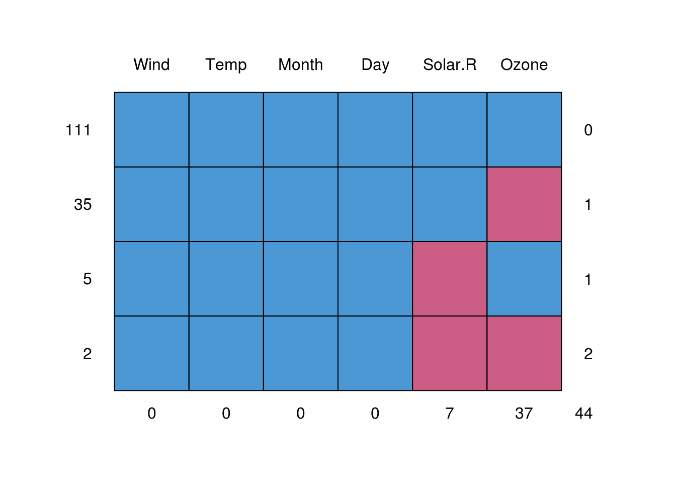
    Wind Temp Month Day Solar.R Ozone
111    1    1     1   1       1     1  0
35     1    1     1   1       1     0  1
5      1    1     1   1       0     1  1
2      1    1     1   1       0     0  2
       0    0     0   0       7    37 44
In this table, md.pattern list the number of cases with particular patterns of missing data.
- Each row describes a misisng data ‘pattern’
- The first column indicates the number of cases
- The central columns indicate whether a particular variable is missing for the pattern (0=missing)
- The last column counts the number of values missing for the pattern
- The final row counts the number of missing values for each variable.
Visualising missingness
Graphics can also be useful to explore patterns in missingness.
rct.data contains data from an RCT of functional imagery training (FIT) for weight loss, which measured outcome (weight in kg) at baseline and two followups (kg1, kg2, kg3). The trial also measured global quality of life (gqol).
As is common, there were some missing data at the follouwp:
fit.data <- readRDS("data/fit-weight.RDS") %>%
  select(kg1, kg2, kg3, age, gqol1)

mice::md.pattern(fit.data)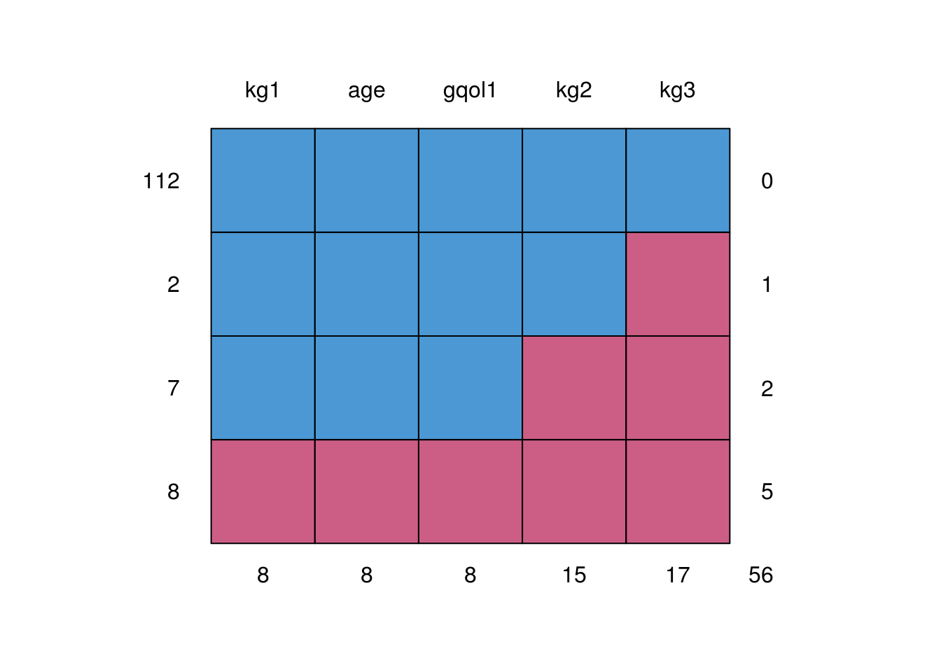
    kg1 age gqol1 kg2 kg3
112   1   1     1   1   1  0
2     1   1     1   1   0  1
7     1   1     1   0   0  2
8     0   0     0   0   0  5
      8   8     8  15  17 56
We might be interested to explore patterns in which observations were missing. Here we use colour to identify missing observations as a function of the data recorded at baseline:
fit.data %>%
  mutate(missing.followup = is.na(kg2)) %>%
  ggplot(aes(kg1, age, color=missing.followup)) +
  geom_point()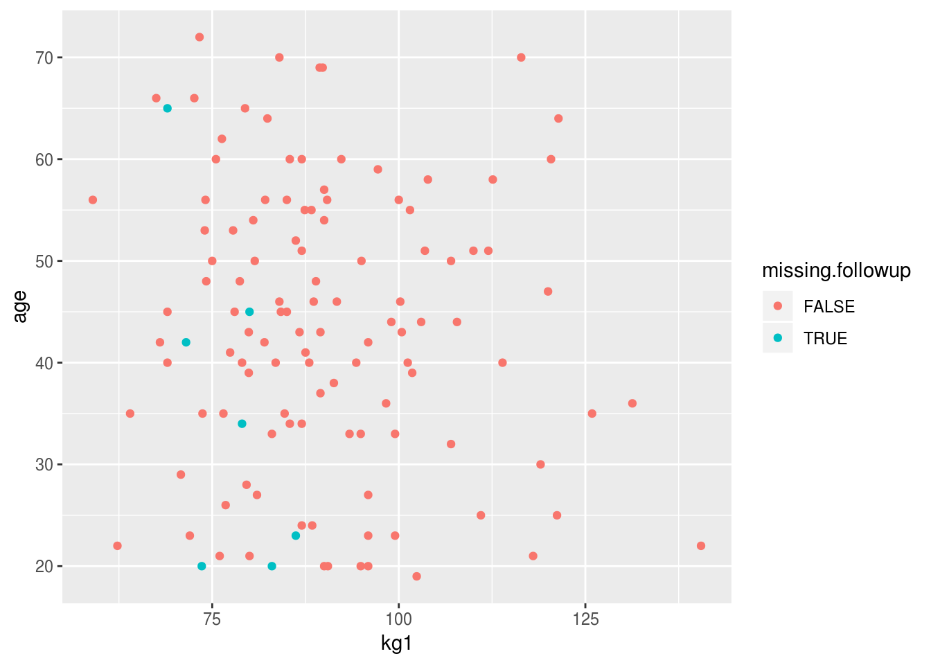
There’s a clear trend here for lighter patients (at baseline) to have more missing data at followup. There’s also a suggestion that younger patients are more likely to have been lost to followup.
If needed, we could perform inferential tests for these differences:
t.test(kg1 ~ is.na(kg2), data=fit.data)

    Welch Two Sample t-test

data:  kg1 by is.na(kg2)
t = 4.7153, df = 11.132, p-value = 0.000614
alternative hypothesis: true difference in means is not equal to 0
95 percent confidence interval:
  7.005116 19.236238
sample estimates:
mean in group FALSE  mean in group TRUE
           90.59211            77.47143
t.test(age ~ is.na(kg2), data=fit.data)

    Welch Two Sample t-test

data:  age by is.na(kg2)
t = 1.2418, df = 6.5246, p-value = 0.2571
alternative hypothesis: true difference in means is not equal to 0
95 percent confidence interval:
 -7.39455 23.25169
sample estimates:
mean in group FALSE  mean in group TRUE
           43.50000            35.57143
However, given the small number of missing values and the post-hoc nature of these analyses these tests are rather underpowered and we might prefer to report and comment on the plot alone.
For some nice missing data visualisation techniques, including those for repeated measures data, see @zhang2015missing.