Structural eqution modelling (SEM)
Combining Path models and CFA to create structural equation models (SEM) allows researchers to combine allow for measurment imperfection whilst also (attempting to) infer information about causation.
SEM involves adding paths to CFA models which are, like predictors in standard regression models, are assumed to be causal in nature; i.e. rather than variables \(x\) and \(y\) simply covarying with one another, we are prepared to make the assumption that \(x\) causes \(y\).
It’s worth pointing out though, right from the offset, that causal relationships drawn from SEM models always dependent on assumptions we are prepared to make when setting up our model. There is nothing magical in the technique that makes allows us to infer causality from non-experimental data (although note SEM can be used for some experimental analyses).
It is only be our substantive knowledge of the domain that makes any kind of causal inference reasonable, and when using SEM the onus is always on us to check our assumptions, provide sensitivity analyses which test alternative causal models, and interpret observational data cautiously.
[Note, there are techniques which use SEM as a means to make stronger kinds of causal statements, for example instrumental variable analysis, but even here, inferring causality still requires that we make strong assumptions about the process which generated our data.
Nonetheless, with these caveats in mind, SEM can be a useful technique to quantify relationships been observed variables where we have measurement error, and especially where we have a theoretical model linking these observations.
Steps to running an SEM
Identify and test the fit of a measurement model. This is a CFA model which includes all of your observed variables, arranged in relation to the latent variables you think generated the data, and where covariances between all these latent variables are included. This step many include many rounds of model fitting and modification.
Ensure your measurement model fits the data adequately before continuing. Test alternative or simplified measurements models and report where these perform well (e.g. are close in fit to your desired model). SEM models that are based on a poorly fitting measurment model will produce parameter estimates that are imprecise, unstable or both, and you should not proceed unless an adequately fitting measrement model is founds (see this nice discussion, which includes relevant references).
Convert your measurement model by removing covariances between latent variables where necessary and including new structural paths. Test model fit, and interpret the paths of interest. Avoid making changes to the measurement part of the model at this stage. Where the model is complex consider adjusting p values to allow for multuple comparisons (if using NHST).
Test alternative models (e.g. with paths removed or reversed). Report where alternatives also fit the data.
In writing up, provide sufficient detail for other researchers to replicate your analyses, and to follow the logic of the ammendments you make. Ideally share your raw data, but at a minimum share the covariance matrix. Report GOF statistics, and follow published reporting guidelines for SEM [@schreiber_reporting_2006]. Always include a diagram of your final model (at the very least).
A worked example: Building from a measurement model to SEM
Imagine we have some data from a study that aimed to test the theory of planned behaviour. Researcher measured exercise and intentions, along with multiple measures of attitudes, social norms and percieved behavioural control.
tpb.df %>% psych::describe(fast=T)| vars | n | mean | sd | min | max | range | se |
| 1 | 469 | -0.00539 | 1.61 | -5.99 | 4.78 | 10.8 | 0.0745 |
| 2 | 459 | 0.117 | 1.22 | -3.17 | 4.18 | 7.35 | 0.057 |
| 3 | 487 | -0.001 | 1.08 | -3.22 | 3.13 | 6.35 | 0.0487 |
| 4 | 487 | 0.078 | 1.53 | -5.04 | 5.43 | 10.5 | 0.0695 |
| 5 | 487 | 0.0376 | 1.22 | -3.76 | 3.61 | 7.37 | 0.0551 |
| 6 | 487 | 0.00863 | 1.11 | -3.21 | 3.11 | 6.33 | 0.0501 |
| 7 | 471 | 0.0261 | 1.1 | -2.94 | 3.14 | 6.08 | 0.0506 |
| 8 | 487 | -0.00329 | 1.35 | -4.13 | 4.03 | 8.16 | 0.061 |
| 9 | 487 | -0.0865 | 1.31 | -4.86 | 4.08 | 8.94 | 0.0593 |
| 10 | 487 | -0.00563 | 1.19 | -3.12 | 3.34 | 6.46 | 0.0537 |
| 11 | 487 | -0.0863 | 1.06 | -3.23 | 3.34 | 6.57 | 0.0481 |
| 12 | 487 | -0.0663 | 1.16 | -4.11 | 3.5 | 7.61 | 0.0525 |
| 13 | 469 | 10.1 | 2.55 | 1.83 | 16.7 | 14.9 | 0.118 |
| 14 | 487 | 80.2 | 18.8 | 15 | 138 | 123 | 0.851 |
There were some missing data, but nothing to suggest a systematic pattern. For the moment we continue with standard methods:
mice::md.pattern(tpb.df)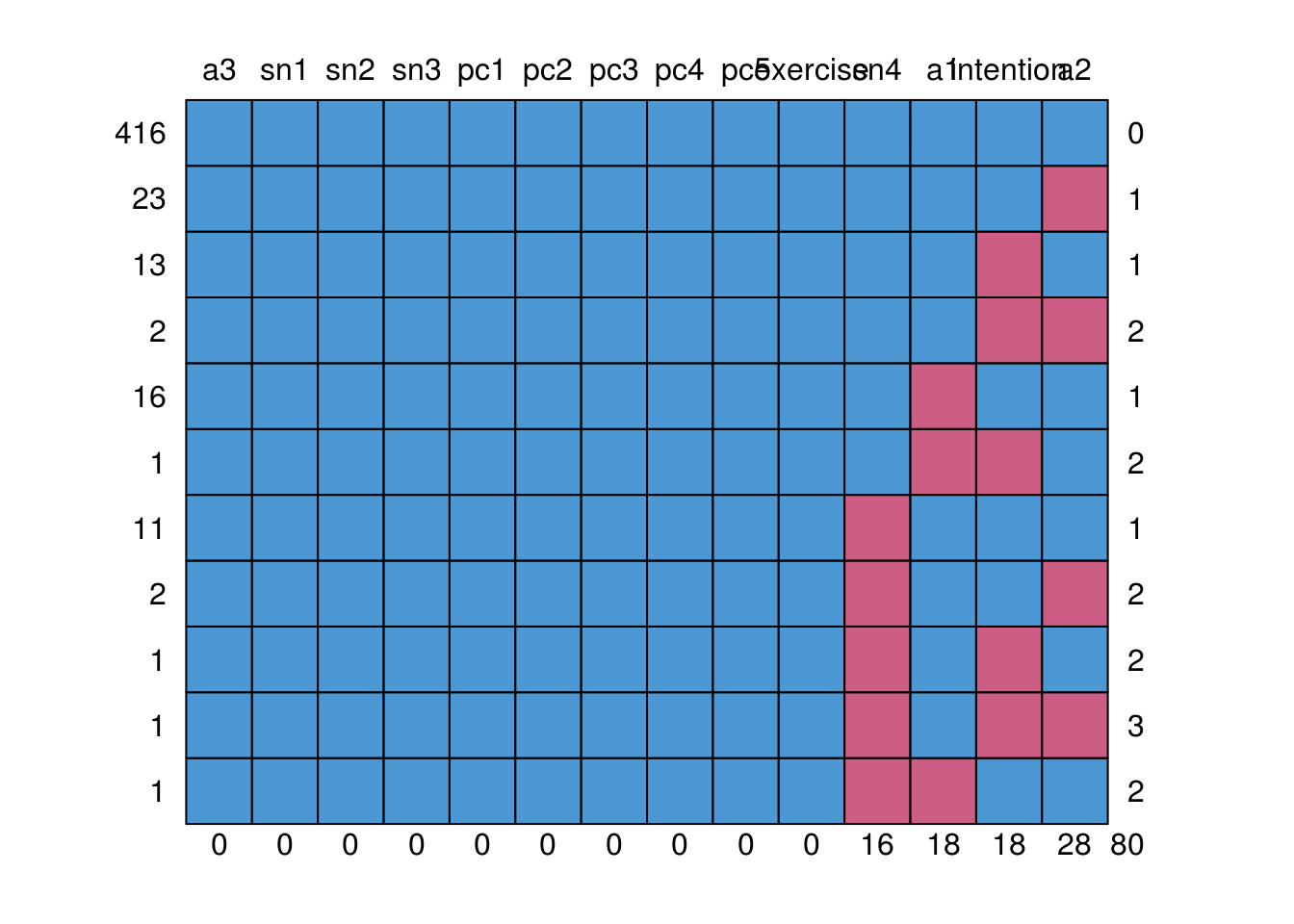
    a3 sn1 sn2 sn3 pc1 pc2 pc3 pc4 pc5 exercise sn4 a1 intention a2
416  1   1   1   1   1   1   1   1   1        1   1  1         1  1  0
23   1   1   1   1   1   1   1   1   1        1   1  1         1  0  1
13   1   1   1   1   1   1   1   1   1        1   1  1         0  1  1
2    1   1   1   1   1   1   1   1   1        1   1  1         0  0  2
16   1   1   1   1   1   1   1   1   1        1   1  0         1  1  1
1    1   1   1   1   1   1   1   1   1        1   1  0         0  1  2
11   1   1   1   1   1   1   1   1   1        1   0  1         1  1  1
2    1   1   1   1   1   1   1   1   1        1   0  1         1  0  2
1    1   1   1   1   1   1   1   1   1        1   0  1         0  1  2
1    1   1   1   1   1   1   1   1   1        1   0  1         0  0  3
1    1   1   1   1   1   1   1   1   1        1   0  0         1  1  2
     0   0   0   0   0   0   0   0   0        0  16 18        18 28 80
We start by fitting a measurement model. The model sytax includes lines with
=~separatatig left and right hand side (to define the latent variables)~~to specify latent covariances
We are not including exercise and intention yet because these are observed
variables only (we don’t have multiple measurements for them) and so they don’t
need to be in the measurement model:
mes.mod <- '
  # the "measurement" part, defining the latent variables
  AT =~ a1 + a2 + a3 + sn1
  SN =~ sn1 + sn2 + sn3 + sn4
  PBC =~ pc1 + pc2 + pc3 + pc4 + pc5

  # note that lavaan automatically includes latent covariances
  # but we can add here anyway to be explicit
  AT ~~ SN
  SN ~~ PBC
  AT ~~ PBC
'
We can fit this model to the data like so:
mes.mod.fit <- cfa(mes.mod, data=tpb.df)
summary(mes.mod.fit)
lavaan 0.6-3 ended normally after 52 iterations

  Optimization method                           NLMINB
  Number of free parameters                         28

                                                  Used       Total
  Number of observations                           429         487

  Estimator                                         ML
  Model Fit Test Statistic                      50.290
  Degrees of freedom                                50
  P-value (Chi-square)                           0.462

Parameter Estimates:

  Information                                 Expected
  Information saturated (h1) model          Structured
  Standard Errors                             Standard

Latent Variables:
                   Estimate  Std.Err  z-value  P(>|z|)
  AT =~
    a1                1.000
    a2                0.471    0.056    8.466    0.000
    a3                0.239    0.042    5.654    0.000
    sn1              -0.145    0.223   -0.651    0.515
  SN =~
    sn1               1.000
    sn2               0.529    0.153    3.456    0.001
    sn3               0.294    0.089    3.300    0.001
    sn4               0.335    0.099    3.383    0.001
  PBC =~
    pc1               1.000
    pc2               0.860    0.098    8.813    0.000
    pc3               0.647    0.081    7.978    0.000
    pc4               0.425    0.069    6.133    0.000
    pc5               0.643    0.081    7.964    0.000

Covariances:
                   Estimate  Std.Err  z-value  P(>|z|)
  AT ~~
    SN                1.488    0.460    3.233    0.001
  SN ~~
    PBC               0.045    0.085    0.525    0.600
  AT ~~
    PBC               0.010    0.086    0.116    0.908

Variances:
                   Estimate  Std.Err  z-value  P(>|z|)
   .a1                0.586    0.195    2.997    0.003
   .a2                1.068    0.086   12.494    0.000
   .a3                1.018    0.072   14.222    0.000
   .sn1               0.870    0.239    3.640    0.000
   .sn2               0.940    0.090   10.404    0.000
   .sn3               1.071    0.077   13.887    0.000
   .sn4               1.028    0.076   13.544    0.000
   .pc1               0.871    0.104    8.401    0.000
   .pc2               1.084    0.100   10.842    0.000
   .pc3               1.018    0.082   12.431    0.000
   .pc4               0.992    0.072   13.690    0.000
   .pc5               1.014    0.081   12.447    0.000
    AT                2.035    0.259    7.859    0.000
    SN                1.873    0.882    2.124    0.034
    PBC               0.888    0.135    6.600    0.000
And we can assess model fit using fitmeasures. Here we select a subset of the
possible fit indices to keep the output manageable.
useful.fit.measures <- c('chisq', 'rmsea', 'cfi', 'aic')
fitmeasures(mes.mod.fit, useful.fit.measures)
    chisq     rmsea       cfi       aic
   50.290     0.004     1.000 16045.276
This model looks pretty good (see the guide to fit indices), but still check modification indices to identify improvements. If they made theoretical sense we might choose to add paths:
modificationindices(mes.mod.fit) %>%
  as_data_frame() %>%
  filter(mi>4) %>%
  arrange(-mi) %>%
pander(caption="Modification indices for the measurement model")| lhs | op | rhs | mi | epc | sepc.lv | sepc.all | sepc.nox |
|---|---|---|---|---|---|---|---|
| AT | =~ | sn2 | 20.39 | 0.5284 | 0.7536 | 0.6226 | 0.6226 |
| sn1 | ~~ | sn2 | 15.04 | -0.4689 | -0.4689 | -0.5184 | -0.5184 |
| AT | =~ | sn4 | 12.49 | -0.3035 | -0.4329 | -0.3891 | -0.3891 |
| a1 | ~~ | sn2 | 8.476 | 0.2457 | 0.2457 | 0.331 | 0.331 |
| sn1 | ~~ | sn4 | 6.54 | 0.216 | 0.216 | 0.2285 | 0.2285 |
| a2 | ~~ | pc5 | 4.098 | -0.1118 | -0.1118 | -0.1074 | -0.1074 |
However, in this case unless we had substantive reasons to add the paths, it would probably be reasonable to continue with the original model.
The measurement model fits, so proceed to SEM
Our SEM model adapts the CFA (measurement model), including additional observed variables (e.g. intention and exercise) and any relevant structural paths:
sem.mod <- '
  # this section identical to measurement model
  AT =~ a1 + a2 + a3 + sn1
  SN =~ sn1 + sn2 + sn3 + sn4
  PBC =~ pc1 + pc2 + pc3 + pc4 + pc5

  # additional structural paths
  intention ~ AT + SN + PBC
  exercise ~ intention
'
We can fit it as before, but now using the sem() function rather than the
cfa() function:
sem.mod.fit <- sem(sem.mod, data=tpb.df)The first thing we do is check the model fit:
fitmeasures(sem.mod.fit, useful.fit.measures)
    chisq     rmsea       cfi       aic
  171.065     0.058     0.929 20638.124
RMSEA is slightly higher than we like, so we can check the modification indices:
sem.mi <- modificationindices(sem.mod.fit) %>%
  as_data_frame() %>%
  arrange(-mi)

sem.mi %>%
  head(6) %>%
pander(caption="Top 6 modification indices for the SEM model")| lhs | op | rhs | mi | epc | sepc.lv | sepc.all | sepc.nox |
|---|---|---|---|---|---|---|---|
| exercise | ~ | PBC | 90.14 | 7.601 | 7.049 | 0.3695 | 0.3695 |
| PBC | ~ | exercise | 89.49 | 0.04938 | 0.05325 | 1.016 | 1.016 |
| intention | ~ | exercise | 47.03 | -0.1233 | -0.1233 | -0.9106 | -0.9106 |
| intention | ~~ | exercise | 47.03 | -16.18 | -16.18 | -0.6779 | -0.6779 |
| AT | =~ | sn2 | 16.14 | 0.5093 | 0.7043 | 0.5855 | 0.5855 |
| pc1 | ~~ | exercise | 15.08 | 2.405 | 2.405 | 0.2205 | 0.2205 |
Interestingly, this model suggests two additional paths involving exercise and
the PBC latent:
sem.mi %>%
  filter(lhs %in% c('exercise', 'PBC') & rhs %in% c('exercise', 'PBC')) %>%
pander()| lhs | op | rhs | mi | epc | sepc.lv | sepc.all | sepc.nox |
|---|---|---|---|---|---|---|---|
| exercise | ~ | PBC | 90.14 | 7.601 | 7.049 | 0.3695 | 0.3695 |
| PBC | ~ | exercise | 89.49 | 0.04938 | 0.05325 | 1.016 | 1.016 |
Of these suggested paths, the largest MI is for the one which says PBC is predicted by exercise. However, the model would also be improved by allowing PBC to predict exercise. Which should we add?
The answer will depend on both previous theory and knowledge of the data.
If it were the case that exercise was measured at a later time point than PBC. In this case the decision is reasonably clear, because the temporal sequencing of observations would determine the most likely path. These data were collected contemporaneously, however, and so we can’t use our design to differentiate the causal possibilities.
Another consideration would be that, by adding a path from exercise to PBC we would make the model non-recursive, and likely non-identified.
A theorist might also argue that because previous studies, and the theory of planned behaviour itself, predict that PBC may exert a direct influence on behaviour, we should add the path with the smaller MI (so allow PBC to predict exercise).
In this case, the best course of action would probably be to report the theoretically implied model, but also test alternative models in which causal relations between the variables are reversed or otherwise altered (along with measures of fit and key parameter estimates). The discussion of your paper would then make the case for your preferred account, but make clear that the data were (most likely) unable to provide a persuasive case either way, and that alternative explanations cannot be ruled out.
Interpreting and presenting key parameters
One of the best ways to present estimates from your final model is in a diagram, because this is intutive and provides a simple way for readers to comprehend the paths implied by your model.
We can automatically generate a plot from a fitted model using semPaths().
Here, the what='std' is requesting standardised parameter estimates be shown.
Adding residuals=F hides variances of observed and latent variables, which are
not of interest here. The line thicknesses are scaled to represent the size
parameter itself:
semPlot::semPaths(sem.mod.fit, what='std', residuals=F)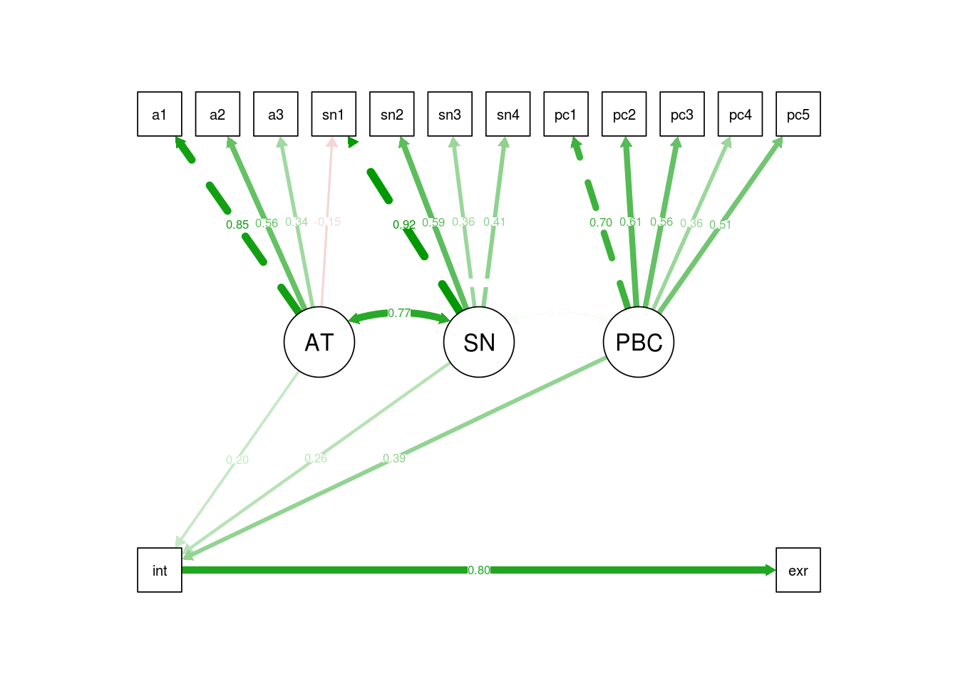
For more information on reporting SEM however, see @schreiber2006reporting.